Tài liệu Đề tài "Gr¨obner geometry of Schubert polynomials " ppt
Bạn đang xem bản rút gọn của tài liệu. Xem và tải ngay bản đầy đủ của tài liệu tại đây (513.46 KB, 75 trang )
Annals of Mathematics
Gr¨obner geometry
of Schubert
polynomials
By Allen Knutson and Ezra Miller
Annals of Mathematics, 161 (2005), 1245–1318
Gr¨obner geometry of Schubert polynomials
By Allen Knutson and Ezra Miller*
Abstract
Given a permutation w ∈ S
n
, we consider a determinantal ideal I
w
whose
generators are certain minors in the generic n × n matrix (filled with inde-
pendent variables). Using ‘multidegrees’ as simple algebraic substitutes for
torus-equivariant cohomology classes on vector spaces, our main theorems de-
scribe, for each ideal I
w
:
• variously graded multidegrees and Hilbert series in terms of ordinary and
double Schubert and Grothendieck polynomials;
• a Gr¨obner basis consisting of minors in the generic n × n matrix;
• the Stanley–Reisner simplicial complex of the initial ideal in terms of
known combinatorial diagrams [FK96], [BB93] associated to permuta-
tions in S
n
; and
• a procedure inductive on weak Bruhat order for listing the facets of this
complex.
We show that the initial ideal is Cohen–Macaulay, by identifying the Stanley–
Reisner complex as a special kind of “subword complex in S
n
”, which we define
generally for arbitrary Coxeter groups, and prove to be shellable by giving an
explicit vertex decomposition. We also prove geometrically a general positivity
statement for multidegrees of subschemes.
Our main theorems provide a geometric explanation for the naturality of
Schubert polynomials and their associated combinatorics. More precisely, we
apply these theorems to:
• define a single geometric setting in which polynomial representatives for
Schubert classes in the integral cohomology ring of the flag manifold are
determined uniquely, and have positive coefficients for geometric reasons;
*AK was partly supported by the Clay Mathematics Institute, Sloan Foundation, and
NSF. EM was supported by the Sloan Foundation and NSF.
1246 ALLEN KNUTSON AND EZRA MILLER
• rederive from a topological perspective Fulton’s Schubert polynomial for-
mula for universal cohomology classes of degeneracy loci of maps between
flagged vector bundles;
• supply new proofs that Schubert and Grothendieck polynomials represent
cohomology and K-theory classes on the flag manifold; and
• provide determinantal formulae for the multidegrees of ladder determi-
nantal rings.
The proofs of the main theorems introduce the technique of “Bruhat in-
duction”, consisting of a collection of geometric, algebraic, and combinatorial
tools, based on divided and isobaric divided differences, that allow one to prove
statements about determinantal ideals by induction on weak Bruhat order.
Contents
Introduction
Part 1. The Gr¨obner geometry theorems
1.1. Schubert and Grothendieck polynomials
1.2. Multidegrees and K-polynomials
1.3. Matrix Schubert varieties
1.4. Pipe dreams
1.5. Gr¨obner geometry
1.6. Mitosis algorithm
1.7. Positivity of multidegrees
1.8. Subword complexes in Coxeter groups
Part 2. Applications of the Gr¨obner geometry theorems
2.1. Positive formulae for Schubert polynomials
2.2. Degeneracy loci
2.3. Schubert classes in flag manifolds
2.4. Ladder determinantal ideals
Part 3. Bruhat induction
3.1. Overview
3.2. Multidegrees of matrix Schubert varieties
3.3. Antidiagonals and mutation
3.4. Lifting Demazure operators
3.5. Coarsening the grading
3.6. Equidimensionality
3.7. Mitosis on facets
3.8. Facets and reduced pipe dreams
3.9. Proofs of Theorems A, B, and C
References
GR
¨
OBNER GEOMETRY OF SCHUBERT POLYNOMIALS
1247
Introduction
The manifold F
n
of complete flags (chains of vector subspaces) in the
vector space C
n
over the complex numbers has historically been a focal point
for a number of distinct fields within mathematics. By definition, F
n
is an
object at the intersection of algebra and geometry. The fact that F
n
can be
expressed as the quotient B\GL
n
of all invertible n×n matrices by its subgroup
of lower triangular matrices places it within the realm of Lie group theory, and
explains its appearance in representation theory. In topology, flag manifolds
arise as fibers of certain bundles constructed universally from complex vector
bundles, and in that context the cohomology ring H
∗
(F
n
)=H
∗
(F
n
; Z)
with integer coefficients Z plays an important role. Combinatorics, especially
related to permutations of a set of cardinality n, aids in understanding the
topology of F
n
in a geometric manner.
To be more precise, the cohomology ring H
∗
(F
n
) equals—in a canonical
way—the quotient of a polynomial ring Z[x
1
, ,x
n
] modulo the ideal gener-
ated by all nonconstant homogeneous functions invariant under permutation
of the indices 1, ,n [Bor53]. This quotient is a free abelian group of rank n!
and has a basis given by monomials dividing
n−1
i=1
x
n−i
i
. This algebraic basis
does not reflect the geometry of flag manifolds as well as the basis of Schubert
classes, which are the cohomology classes of Schubert varieties X
w
, indexed
by permutations w ∈ S
n
[Ehr34]. The Schubert variety X
w
consists of flags
V
0
⊂ V
1
⊂···⊂V
n−1
⊂ V
n
whose intersections V
i
∩ C
j
have dimensions deter-
mined in a certain way by w, where C
j
is spanned by the first j basis vectors
of C
n
.
A great deal of research has grown out of attempts to understand
the connection between the algebraic basis of monomials and the geometric
basis of Schubert classes [X
w
] in the cohomology ring H
∗
(F
n
). For this pur-
pose, Lascoux and Sch¨utzenberger singled out Schubert polynomials S
w
∈
Z[x
1
, ,x
n
] as representatives for Schubert classes [LS82a], relying in large
part on earlier work of Demazure [Dem74] and Bernstein–Gel
fand–Gel
fand
[BGG73]. Lascoux and Sch¨utzenberger justified their choices with algebra and
combinatorics, whereas the earlier work had been in the context of geometry.
This paper bridges the algebra and combinatorics of Schubert polynomials on
the one hand with the geometry of Schubert varieties on the other. In the
process, it brings a new perspective to problems in commutative algebra con-
cerning ideals generated by minors of generic matrices.
Combinatorialists have in fact recognized the intrinsic interest of Schubert
polynomials S
w
for some time, and have therefore produced a wealth of inter-
pretations for their coefficients. For example, see [Ber92], [Mac91, App. Ch. IV,
by N. Bergeron], [BJS93], [FK96], [FS94], [Koh91], and [Win99]. Geometers,
on the other hand, who take for granted Schubert classes [X
w
] in cohomol-
1248 ALLEN KNUTSON AND EZRA MILLER
ogy of flag manifold F
n
, generally remain less convinced of the naturality of
Schubert polynomials, even though these polynomials arise in certain univer-
sal geometric contexts [Ful92], and there are geometric proofs of positivity for
their coefficients [BS02], [Kog00].
Our primary motivation for undertaking this project was to provide a
geometric context in which both (i) polynomial representatives for Schubert
classes [X
w
] in the integral cohomology ring H
∗
(F
n
) are uniquely singled out,
with no choices other than a Borel subgroup of the general linear group GL
n
C;
and (ii) it is geometrically obvious that these representatives have nonnegative
coefficients. That our polynomials turn out to be the Schubert polynomials is
a testament to the naturality of Schubert polynomials; that our geometrically
positive formulae turn out to reproduce known combinatorial structures is a
testament to the naturality of the combinatorics previously unconvincing to
geometers.
The kernel of our idea was to translate ordinary cohomological statements
concerning Borel orbit closures on the flag manifold F
n
into equivariant-
cohomological statements concerning double Borel orbit closures on the n × n
matrices M
n
. Briefly, the preimage
˜
X
w
⊆ GL
n
of a Schubert variety X
w
⊆
F
n
= B\GL
n
is an orbit closure for the action of B×B
+
, where B and B
+
are
the lower and upper triangular Borel subgroups of GL
n
acting by multiplication
on the left and right. When
X
w
⊆ M
n
is the closure of
˜
X
w
and T is the torus
in B, the T -equivariant cohomology class [
X
w
]
T
∈ H
∗
T
(M
n
)=Z[x
1
, ,x
n
]
is our polynomial representative. It has positive coefficients because there is
a T -equivariant flat (Gr¨obner) degeneration
X
w
L
w
to a union of coordi-
nate subspaces L ⊆ M
n
. Each subspace L ⊆L
w
has equivariant cohomology
class [L]
T
∈ H
∗
T
(M
n
) that is a monomial in x
1
, ,x
n
, and the sum of these is
[
X
w
]
T
. Our obviously positive formula is thus simply
[
X
w
]
T
=[L
w
]
T
=
L∈L
w
[L]
T
.(1)
In fact, one need not actually produce a degeneration of X
w
to a union
of coordinate subspaces: the mere existence of such a degeneration is enough
to conclude positivity of the cohomology class [
X
w
]
T
, although if the limit is
nonreduced then subspaces must be counted according to their (positive) multi-
plicities. This positivity holds quite generally for sheaves on vector spaces with
torus actions, because existence of degenerations is a standard consequence of
Gr¨obner basis theory. That being said, in our main results we identify a partic-
ularly natural degeneration of the matrix Schubert variety
X
w
, with reduced
and Cohen–Macaulay limit L
w
, in which the subspaces have combinatorial in-
terpretations, and (1) coincides with the known combinatorial formula [BJS93],
[FS94] for Schubert polynomials.
GR
¨
OBNER GEOMETRY OF SCHUBERT POLYNOMIALS
1249
The above argument, as presented, requires equivariant cohomology
classes associated to closed subvarieties of noncompact spaces such as M
n
,
the subtleties of which might be considered unpalatable, and certainly require
characteristic zero. Therefore we instead develop our theory in the context
of multidegrees, which are algebraically defined substitutes. In this setting,
equivariant considerations for matrix Schubert varieties
X
w
⊆ M
n
guide our
path directly toward multigraded commutative algebra for the Schubert deter-
minantal ideals I
w
cutting out the varieties X
w
.
Example. Let w = 2143 be the permutation in the symmetric group S
4
sending 1 → 2, 2 → 1, 3 → 4 and 4 → 3. The matrix Schubert variety X
2143
is the set of 4 × 4 matrices Z =(z
ij
) whose upper-left entry is zero, and whose
upper-left 3 × 3 block has rank at most two. The equations defining
X
2143
are
the vanishing of the determinants
z
11
,
z
11
z
12
z
13
z
21
z
22
z
23
z
31
z
32
z
33
= −z
13
z
22
z
31
+
.
When we Gr¨obner-degenerate the matrix Schubert variety to the scheme de-
fined by the initial ideal z
11
, −z
13
z
22
z
31
, we get a union L
2143
of three coor-
dinate subspaces
L
11,13
,L
11,22
, and L
11,31
, with ideals z
11
,z
13
, z
11
,z
22
, and z
11
,z
31
.
In the Z
n
-grading where z
ij
has weight x
i
, the multidegree of L
i
1
j
1
,i
2
j
2
equals
x
i
1
x
i
2
. Our “obviously positive” formula (1) for S
2143
(x) says that [X
2143
]
T
=
x
2
1
+ x
1
x
2
+ x
1
x
3
.
Pictorially, we represent the subspaces L
11,13
, L
11,22
, and L
11,31
inside
L
2143
as subsets
z
11
,z
13
=
+ +
, z
11
,z
22
=
+
+
, z
11
,z
31
=
+
+
of the 4×4 grid, or equivalently as “pipe dreams” with crosses and “elbow
joints”
✆✞
instead of boxes with + or nothing, respectively (imagine
✆✞
filling
the lower right corners):
1234
2
✆✞ ✆
1
✆✞ ✆✞ ✆
4
✆✞ ✆
3
✆
1234
2
✆✞ ✆✞ ✆
1
✆✞ ✆
4
✆✞ ✆
3
✆
1234
2
✆✞ ✆✞ ✆
1
✆✞ ✆✞ ✆
4
✆
3
✆
These are the three “reduced pipe dreams”, or “planar histories”, for w = 2143
[FK96], and so we recover the combinatorial formula for S
w
(x) from [BJS93],
[FS94].
1250 ALLEN KNUTSON AND EZRA MILLER
Our main ‘Gr¨obner geometry’ theorems describe, for every matrix
Schubert variety
X
w
:
• its multidegree and Hilbert series, in terms of Schubert and Grothendieck
polynomials (Theorem A);
• a Gr¨obner basis consisting of minors in its defining ideal I
w
(Theorem B);
• the Stanley–Reisner complex L
w
of its initial ideal J
w
, which we prove
is Cohen–Macaulay, in terms of pipe dreams and combinatorics of S
n
(Theorem B); and
• an inductive irredundant algorithm (‘mitosis’) on weak Bruhat order for
listing the facets of L
w
(Theorem C).
Gr¨obner geometry of Schubert polynomials thereby provides a geometric ex-
planation for the naturality of Schubert polynomials and their associated com-
binatorics.
The divided and isobaric divided differences used by Lascoux and
Sch¨utzenberger to define Schubert and Grothendieck polynomials inductively
[LS82a], [LS82b] were originally invented by virtue of their geometric interpre-
tation by Demazure [Dem74] and Bernstein–Gel
fand–Gel
fand [BGG73]. The
heart of our proof of the Gr¨obner geometry theorem for Schubert polynomi-
als captures the divided and isobaric divided differences in their algebraic and
combinatorial manifestations. Both manifestations are positive: one in terms
of the generators of the initial ideal J
w
and the monomials outside J
w
, and the
other in terms of certain combinatorial diagrams (reduced pipe dreams) associ-
ated to permutations by Fomin–Kirillov [FK96]. Taken together, the geomet-
ric, algebraic, and combinatorial interpretations provide a powerful inductive
method, which we call Bruhat induction, for working with determinantal ideals
and their initial ideals, as they relate to multigraded cohomological and combi-
natorial invariants. In particular, Bruhat induction applied to the facets of L
w
proves a geometrically motivated substitute for Kohnert’s conjecture [Koh91].
At present, “almost all of the approaches one can choose for the investi-
gation of determinantal rings use standard bitableaux and the straightening
law” [BC01, p. 3], and are thus intimately tied to the Robinson–Schensted–
Knuth (RSK) correspondence. Although Bruhat induction as developed here
may seem similar in spirit to RSK, in that both allow one to work directly
with vector space bases in the quotient ring, Bruhat induction contrasts with
methods based on RSK in that it compares standard monomials of different
ideals inductively on weak Bruhat order, instead of comparing distinct bases
associated to the same ideal, as RSK does. Consequently, Bruhat induction
encompasses a substantially larger class of determinantal ideals.
GR
¨
OBNER GEOMETRY OF SCHUBERT POLYNOMIALS
1251
Bruhat induction, as well as the derivation of the main theorems concern-
ing Gr¨obner geometry of Schubert polynomials from it, relies on two general
results concerning
• positivity of multidegrees—that is, positivity of torus-equivariant coho-
mology classes represented by subschemes or coherent sheaves on vector
spaces (Theorem D); and
• shellability of certain simplicial complexes that reflect the nature of re-
duced subwords of words in Coxeter generators for Coxeter groups (The-
orem E).
The latter of these allows us to approach the combinatorics of Schubert and
Grothendieck polynomials from a new perspective, namely that of simplicial
topology. More precisely, our proof of shellability for the initial complex L
w
draws on previously unknown combinatorial topological aspects of reduced ex-
pressions in symmetric groups, and more generally in arbitrary Coxeter groups.
We touch relatively briefly on this aspect of the story here, only proving what
is essential for the general picture in the present context, and refer the reader
to [KnM04] for a complete treatment, including applications to Grothendieck
polynomials.
Organization. Our main results, Theorems A, B, C, D, and E, appear
in Sections 1.3, 1.5, 1.6, 1.7, and 1.8, respectively. The sections in Part 1 are
almost entirely expository in nature, and serve not merely to define all objects
appearing in the central theorems, but also to provide independent motivation
and examples for the theories they describe. For each of Theorems A, B,
C, and E, we develop before it just enough prerequisites to give a complete
statement, while for Theorem D we first provide a crucial characterization of
multidegrees, in Theorem 1.7.1.
Readers seeing this paper for the first time should note that Theorems A,
B, and D are core results, not to be overlooked on a first pass through. Theo-
rems C and E are less essential to understanding the main point as outlined in
the introduction, but still fundamental for the combinatorics of Schubert poly-
nomials as derived from geometry via Bruhat induction (which is used to prove
Theorems A and B), and for substantiating the naturality of the degeneration
in Theorem B.
The paper is structured logically as follows. There are no proofs in Sec-
tions 1.1–1.6 except for a few easy lemmas that serve the exposition. The
complete proof of Theorems A, B, and C must wait until the last section of
Part 3 (Section 3.9), because these results rely on Bruhat induction. Sec-
tion 3.9 indicates which parts of the theorems from Part 1 imply the others,
while gathering the results from Part 3 to prove those required parts. In con-
1252 ALLEN KNUTSON AND EZRA MILLER
trast, the proofs of Theorems D and E in Sections 1.7 and 1.8 are completely
self-contained, relying on nothing other than definitions. Results of Part 1 are
used freely in Part 2 for applications to consequences not found or only briefly
mentioned in Part 1. The development of Bruhat induction in Part 3 depends
only on Section 1.7 and definitions from Part 1.
In terms of content, Sections 1.1, 1.2, and 1.4, as well as the first half of
Section 1.3, review known definitions, while the other sections in Part 1 intro-
duce topics appearing here for the first time. In more detail, Section 1.1 recalls
the Schubert and Grothendieck polynomials of Lascoux and Sch¨utzenberger
via divided differences and their isobaric relatives. Then Section 1.2 reviews
K-polynomials and multidegrees, which are rephrased versions of the equiv-
ariant multiplicities in [BB82], [BB85], [Jos84], [Ros89]. We start Section 1.3
by introducing matrix Schubert varieties and Schubert determinantal ideals,
which are due (in different language) to Fulton [Ful92]. This discussion cul-
minates in the statement of Theorem A, giving the multidegrees and K-
polynomials of matrix Schubert varieties.
We continue in Section 1.4 with some combinatorial diagrams that we
call ‘reduced pipe dreams’, associated to permutations. These were invented
by Fomin and Kirillov and studied by Bergeron and Billey, who called them
‘rc-graphs’. Section 1.5 begins with the definition of ‘antidiagonal’ squarefree
monomial ideals, and proceeds to state Theorem B, which describes Gr¨obner
bases and initial ideals for matrix Schubert varieties in terms of reduced pipe
dreams. Section 1.6 defines our combinatorial ‘mitosis’ rule for manipulating
subsets of the n × n grid, and describes in Theorem C how mitosis generates
all reduced pipe dreams.
Section 1.7 works with multidegrees in the general context of a positive
multigrading, proving the characterization Theorem 1.7.1 and then its conse-
quence, the Positivity Theorem D. Also in a general setting—that of arbitrary
Coxeter groups—we define ‘subword complexes’ in Section 1.8, and prove their
vertex-decomposability in Theorem E.
Our most important application, in Section 2.1, consists of the geomet-
rically positive formulae for Schubert polynomials that motivated this paper.
Other applications include connections with Fulton’s theory of degeneracy loci
in Section 2.2, relations between our multidegrees and K-polynomials on n× n
matrices with classical cohomological theories on the flag manifold in Sec-
tion 2.3, and comparisons in Section 2.4 with the commutative algebra litera-
ture on determinantal ideals.
Part 3 demonstrates how the method of Bruhat induction works geo-
metrically, algebraically, and combinatorially to provide full proofs of Theo-
rems A, B, and C. We postpone the detailed overview of Part 3 until Sec-
tion 3.1, although we mention here that the geometric Section 3.2 has a rather
different flavor from Sections 3.3–3.8, which deal mostly with the combinatorial
GR
¨
OBNER GEOMETRY OF SCHUBERT POLYNOMIALS
1253
commutative algebra spawned by divided differences, and Section 3.9, which
collects Part 3 into a coherent whole in order to prove Theorems A, B, and C.
Generally speaking, the material in Part 3 is more technical than earlier parts.
We have tried to make the material here as accessible as possible to com-
binatorialists, geometers, and commutative algebraists alike. In particular, ex-
cept for applications in Part 2, we have assumed no specific knowledge of the
algebra, geometry, or combinatorics of flag manifolds, Schubert varieties, Schu-
bert polynomials, Grothendieck polynomials, or determinantal ideals. Many
of our examples interpret the same underlying data in varying contexts, to
highlight and contrast common themes. In particular this is true of Exam-
ples 1.3.5, 1.4.2, 1.4.6, 1.5.3, 1.6.2, 1.6.3, 3.3.6, 3.3.7, 3.4.2, 3.4.7, 3.4.8, 3.7.4,
3.7.6, and 3.7.10.
Conventions. Throughout this paper, k is an arbitary field. In partic-
ular, we impose no restrictions on its characteristic. Furthermore, although
some geometric statements or arguments may seem to require that k be alge-
braically closed, this hypothesis could be dispensed with formally by resorting
to sufficiently abstruse language.
We consciously chose our notational conventions (with considerable effort)
to mesh with those of [Ful92], [LS82a], [FK94], [HT92], and [BB93] concerning
permutations (w
T
versus w), the indexing on (matrix) Schubert varieties and
polynomials (open orbit corresponds to identity permutation and smallest orbit
corresponds to long word), the placement of one-sided ladders (in the north-
west corner as opposed to the southwest), and reduced pipe dreams. These
conventions dictated our seemingly idiosyncratic choices of Borel subgroups as
well as the identification F
n
∼
=
B\GL
n
as the set of right cosets, and resulted
in our use of row vectors in k
n
instead of the usual column vectors. That there
even existed consistent conventions came as a relieving surprise.
Acknowledgements. The authors are grateful to Bernd Sturmfels, who took
part in the genesis of this project, and to Misha Kogan, as well as to Sara Billey,
Francesco Brenti, Anders Buch, Christian Krattenthaler, Cristian Lenart, Vic
Reiner, Rich´ard Rim´anyi, Anne Schilling, Frank Sottile, and Richard Stanley
for inspiring conversations and references. Nantel Bergeron kindly provided
L
A
T
E
X macros for drawing pipe dreams.
Part 1. The Gr¨obner geometry theorems
1.1. Schubert and Grothendieck polynomials
We write all permutations in one-line (not cycle) notation, where w =
w
1
w
n
sends i → w
i
. Set w
0
= n 321 equal to the long permutation
reversing the order of 1, ,n.
1254 ALLEN KNUTSON AND EZRA MILLER
Definition 1.1.1. Let R be a commutative ring, and x = x
1
, ,x
n
inde-
pendent variables. The i
th
divided difference operator ∂
i
takes each polynomial
f ∈ R[x]to
∂
i
f(x
1
,x
2
, )=
f(x
1
,x
2
, ,) − f(x
1
, ,x
i−1
,x
i+1
,x
i
,x
i+2
, )
x
i
− x
i+1
.
The Schubert polynomial for w ∈ S
n
is defined by the recursion
S
ws
i
(x)=∂
i
S
w
(x)
whenever length(ws
i
) < length(w), and the initial condition S
w
0
(x)=
n
i=1
x
n−i
i
∈ Z[x]. The double Schubert polynomials S
w
(x, y) are defined by
the same recursion, but starting from S
w
0
(x, y)=
i+j≤n
(x
i
− y
j
) ∈ Z[y][x].
In the definition of S
w
(x, y), the operator ∂
i
is to act only on the x vari-
ables and not on the y variables. Checking monomial by monomial verifies that
x
i
− x
i+1
divides the numerator of ∂
i
(f), and so ∂
i
(f) is again a polynomial,
homogeneous of degree d − 1iff is homogeneous of degree d.
Example 1.1.2. Here are all of the Schubert polynomials for permutations
in S
3
, along with the rules for applying divided differences.
x
2
1
x
2
∂
2
∂
1
x
2
1
x
1
x
2
∂
2
↓
∂
1
∂
2
↓
∂
1
0 x
1
+ x
2
x
1
0
∂
1
∂
2
∂
1
∂
2
010
The recursion for both single and double Schubert polynomials can be
summarized as
S
w
= ∂
i
k
···∂
i
1
S
w
0
,
where w
0
w = s
i
1
···s
i
k
and length(w
0
w)=k. The condition length(w
0
w)=k
means by definition that k is minimal, so that w
0
w = s
i
1
···s
i
k
is a reduced
expression for w
0
w. It is not immediately obvious from Definition 1.1.1 that
S
w
is well-defined, but it follows from the fact that divided differences satisfy
the Coxeter relations, ∂
i
∂
i+1
∂
i
= ∂
i+1
∂
i
∂
i+1
and ∂
i
∂
i
= ∂
i
∂
i
when |i − i
|≥2.
Divided differences arose geometrically in work of Demazure [Dem74] and
Bernstein–Gel
fand–Gel
fand [BGG73], where they reflected a ‘Bott–Samelson
crank’: form a P
1
bundle over a Schubert variety and smear it out onto the flag
manifold F
n
to get a Schubert variety of dimension 1 greater than before. In
their setting, the variables x represented Chern classes of standard line bundles
L
1
, ,L
n
on F
n
, where the fiber of L
i
over a flag F
0
⊂···⊂F
n
is the dual
GR
¨
OBNER GEOMETRY OF SCHUBERT POLYNOMIALS
1255
vector space (F
i
/F
i−1
)
∗
. The divided differences acted on the cohomology ring
H
∗
(F
n
), which is the quotient of Z[x] modulo the ideal generated by sym-
metric functions with no constant term [Bor53]. The insight of Lascoux and
Sch¨utzenberger in [LS82a] was to impose a stability condition on the collec-
tion of polynomials S
w
that defines them uniquely among representatives for
the cohomology classes of Schubert varieties. More precisely, although Def-
inition 1.1.1 says that w lies in S
n
, the number n in fact plays no role: if
w
N
∈ S
N
for n ≥ N agrees with w on 1, ,n and fixes n +1, ,N, then
S
w
N
(x
1
, ,x
N
)=S
w
(x
1
, ,x
n
).
The ‘double’ versions represent Schubert classes in equivariant cohomology
for the Borel group action on F
n
. As the ordinary Schubert polynomials are
much more common in the literature than double Schubert polynomials, we
have phrased many of our coming results both in terms of Schubert polynomials
as well as double Schubert polynomials. This choice has the advantage of
demonstrating how the notation simplifies in the single case.
Schubert polynomials have their analogues in K-theory of F
n
, where
the recurrence uses a “homogenized” operator (sometimes called an isobaric
divided difference operator):
Definition 1.1.3. Let R be a commutative ring. The i
th
Demazure oper-
ator
∂
i
: R[[x]] → R[[x]] sends a power series f (x)to
x
i+1
f(x
1
, ,x
n
) − x
i
f(x
1
, ,x
i−1
,x
i+1
,x
i
,x
i+2
, ,x
n
)
x
i+1
− x
i
= −∂
i
(x
i+1
f).
The Grothendieck polynomial G
w
(x) is obtained recursively from the “top”
Grothendieck polynomial G
w
0
(x):=
n
i=1
(1 − x
i
)
n−i
via the recurrence
G
ws
i
(x)=∂
i
G
w
(x)
whenever length(ws
i
) < length(w). The double Grothendieck polynomials are
defined by the same recurrence, but start from G
w
0
(x, y):=
i+j≤n
(1−x
i
y
−1
j
).
As with divided differences, one can check directly that Demazure oper-
ators
∂
i
take power series to power series, and satisfy the Coxeter relations.
Lascoux and Sch¨utzenberger [LS82b] showed that Grothendieck polynomials
enjoy the same stability property as do Schubert polynomials; we shall rederive
this fact directly from Theorem A in Section 2.3 (Lemma 2.3.2), where we also
construct the bridge from Gr¨obner geometry of Schubert and Grothendieck
polynomials to classical geometry on flag manifolds.
Schubert polynomials represent data that are leading terms for the richer
structure encoded by Grothendieck polynomials.
1256 ALLEN KNUTSON AND EZRA MILLER
Lemma 1.1.4. The Schubert polynomial S
w
(x) is the sum of all lowest-
degree terms in G
w
(1 − x), where (1 − x)=(1− x
1
, ,1 − x
n
). Similarly, the
double Schubert polynomial S
w
(x, y) is the sum of all lowest-degree terms in
G
w
(1 − x, 1 − y).
Proof. Assuming f(1 − x) is homogeneous, plugging 1 − x for x into the
first displayed equation in Definition 1.1.3 and taking the lowest degree terms
yields ∂
i
f(1 − x). Since S
w
0
is homogeneous, the result follows by induction
on length(w
0
w).
Although the Demazure operators are usually applied only to polynomi-
als in x, it will be crucial in our applications to use them on power series
in x. We shall also use the fact that, since the standard denominator f(x)=
n
i=1
(1−x
i
)
n
for Z
n
-graded Hilbert series over k[z] is symmetric in x
1
, ,x
n
,
applying
∂
i
to a Hilbert series g/f simplifies: ∂
i
(g/f)=(∂
i
g)/f . This can easily
be checked directly. The same comment applies when f(x)=
n
i,j=1
(1−x
i
/y
j
)
is the standard denominator for Z
2n
-graded Hilbert series.
1.2. Multidegrees and K-polynomials
Our first main theorem concerns cohomological and K-theoretic invariants
of matrix Schubert varieties, which are given by multidegrees and
K-polynomials, respectively. We work with these here in the setting of a
polynomial ring k[z]inm variables z = z
1
, ,z
m
, with a grading by Z
d
in
which each variable z
i
has exponential weight wt(z
i
)=t
a
i
for some vector
a
i
=(a
i1
, ,a
id
) ∈ Z
d
, where t = t
1
, ,t
d
. We call a
i
the ordinary weight
of z
i
, and sometimes write a
i
= deg(z
i
)=a
i1
t
1
+ ···+ a
id
t
d
. It is useful to
think of this as the logarithm of the Laurent monomial t
a
i
.
Example 1.2.1. Our primary concern is the case z =(z
ij
)
n
i,j=1
with vari-
ous gradings, in which the different kinds of weights are:
grading
ZZ
n
Z
2n
Z
n
2
exponential weight of z
ij
tx
i
x
i
/y
j
z
ij
ordinary weight of z
ij
tx
i
x
i
− y
j
z
ij
The exponential weights are Laurent monomials that we treat as elements in
the group rings Z[t
±1
], Z[x
±1
], Z[x
±1
, y
±1
], Z[z
±1
] of the grading groups. The
ordinary weights are linear forms that we treat as elements in the integral
symmetric algebras Z[t] = Sym
.
Z
(Z), Z[x] = Sym
.
Z
(Z
n
), Z[x, y] = Sym
.
Z
(Z
2n
),
Z[z] = Sym
.
Z
(Z
n
2
) of the grading groups.
GR
¨
OBNER GEOMETRY OF SCHUBERT POLYNOMIALS
1257
Every finitely generated Z
d
-graded module Γ =
a∈
Z
d
Γ
a
over k[z] has a
free resolution
E
.
:0←E
0
←E
1
←···←E
m
← 0, where E
i
=
β
i
j=1
k[z](−b
ij
)
is graded, with the j
th
summand of E
i
generated in Z
d
-graded degree b
ij
.
Definition 1.2.2. The K-polynomial of Γ is K(Γ; t)=
i
(−1)
i
j
t
b
ij
.
Geometrically, the K-polynomial of Γ represents the class of the sheaf
˜
Γonk
m
in equivariant K-theory for the action of the d-torus whose weight
lattice is Z
d
. Algebraically, when the Z
d
-grading is positive, meaning that the
ordinary weights a
1
, ,a
d
lie in a single open half-space in Z
d
, the vector
space dimensions dim
k
(Γ
a
) are finite for all a ∈ Z
d
, and the K-polynomial
of Γ is the numerator of its Z
d
-graded Hilbert series H(Γ; t):
H(Γ; t):=
a∈
Z
d
dim
k
(Γ
a
) · t
a
=
K(Γ; t)
m
i=1
(1 − wt(z
i
))
.
We shall only have a need to consider positive multigradings in this paper.
Given any Laurent monomial t
a
= t
a
1
1
···t
a
d
d
, the rational function
d
j=1
(1 − t
j
)
a
j
can be expanded as a well-defined (that is, convergent in the
t-adic topology) formal power series
d
j=1
(1 − a
j
x
j
+ ···)int. Doing the
same for each monomial in an arbitrary Laurent polynomial K(t) results in a
power series denoted by K(1 − t).
Definition 1.2.3. The multidegree of a Z
d
-graded k[z]-module Γ is the sum
C(Γ; t) of the lowest degree terms in K(Γ; 1−t). If Γ = k[z]/I is the coordinate
ring of a subscheme X ⊆ k
m
, then we may also write [X]
Z
d
or C(X; t) to mean
C(Γ; t).
Geometrically, multidegrees are just an algebraic reformulation of torus-
equivariant cohomology of affine space, or equivalently the equivariant Chow
ring [Tot99], [EG98]. Multidegrees originated in [BB82], [BB85] as well as
[Jos84], and are called equivariant multiplicities in [Ros89].
Example 1.2.4. Let n = 2 in Example 1.2.1, and set
Γ=k
z
11
z
12
z
21
z
22
/z
11
,z
22
.
Then
K(Γ; z)=(1− z
11
)(1 − z
22
) and K(Γ; x, y)=(1− x
1
/y
1
)(1 − x
2
/y
2
)
1258 ALLEN KNUTSON AND EZRA MILLER
because of the Koszul resolution. Thus K(Γ; 1 − z)=z
11
z
22
= C(Γ; z), and
K(Γ; 1 − x, 1 − y)=(x
1
− y
1
+ x
1
y
1
− y
2
1
+ ···)(x
2
− y
2
+ x
2
y
2
− y
2
2
+ ···),
whose sum of lowest degree terms is C(Γ; x, y)=(x
1
− y
1
)(x
2
− y
2
).
The letters C and K stand for ‘cohomology’ and ‘K-theory’, the rela-
tion between them (‘take lowest degree terms’) reflecting the Grothendieck–
Riemann–Roch transition from K-theory to its associated graded ring. When
k is the complex field C, the (Laurent) polynomials denoted by C and K are
honest torus-equivariant cohomology and K-classes on C
m
.
1.3. Matrix Schubert varieties
Let M
n
be the variety of n×n matrices over k, with coordinate ring k[z]in
indeterminates {z
ij
}
n
i,j=1
. Throughout the paper, q and p will be integers with
1 ≤ q,p ≤ n, and Z will stand for an n × n matrix. Most often, Z will be the
generic matrix of variables (z
ij
), although occasionally Z will be an element
of M
n
. Denote by Z
q×p
the northwest q × p submatrix of Z. For instance,
given a permutation w ∈ S
n
, the permutation matrix w
T
with ‘1’ entries in
row i and column w(i) has upper-left q × p submatrix with rank given by
rank(w
T
q×p
)=#{(i, j) ≤ (q, p) | w(i)=j},
the number of ‘1’ entries in the submatrix w
T
q×p
.
The class of determinantal ideals in the following definition was identified
by Fulton in [Ful92], though in slightly different language.
Definition 1.3.1. Let w ∈ S
n
be a permutation. The Schubert determi-
nantal ideal I
w
⊂ k[z] is generated by all minors in Z
q×p
of size 1+ rank(w
T
q×p
)
for all q, p, where Z =(z
ij
) is the matrix of variables.
The subvariety of M
n
cut out by I
w
is the central geometric object in this
paper.
Definition 1.3.2. Let w ∈ S
n
. The matrix Schubert variety X
w
⊆ M
n
consists of the matrices Z ∈ M
n
such that rank(Z
q×p
) ≤ rank(w
T
q×p
) for all q,p.
Example 1.3.3. The smallest matrix Schubert variety is
X
w
0
, where w
0
is the long permutation n ··· 2 1 reversing the order of 1, ,n. The variety
X
w
0
is just the linear subspace of lower-right-triangular matrices; its ideal is
z
ij
| i + j ≤ n.
GR
¨
OBNER GEOMETRY OF SCHUBERT POLYNOMIALS
1259
Example 1.3.4. Five of the six 3 × 3 matrix Schubert varieties are linear
subspaces:
I
123
=0 X
123
= M
3
I
213
= z
11
X
213
= {Z ∈ M
3
| z
11
=0}
I
231
= z
11
,z
12
X
231
= {Z ∈ M
3
| z
11
= z
12
=0}
I
231
= z
11
,z
21
X
312
= {Z ∈ M
3
| z
11
= z
21
=0}
I
321
= z
11
,z
12
,z
21
X
321
= {Z ∈ M
3
| z
11
= z
12
= z
21
=0}.
The remaining permutation, w = 132, has
I
132
= z
11
z
22
− z
12
z
21
, X
132
= {Z ∈ M
3
| rank(Z
2×2
) ≤ 1},
so that
X
132
is the set of matrices whose upper-left 2 × 2 block is singular.
Example 1.3.5. Let w = 13865742, so that w
T
is given by replacing each
∗ by 1 in the left matrix below.
∗
∗
∗
∗
∗
∗
∗
∗
⇒
1 1 1 1 1 1 1 1
1 1
1 1
1 1
1 1
1 1
1 1
1
,
2 2 2 2 2 2 2 2
2 2 2 2 2 2 2 2
2 2 2 2 2 2 2
2 2 2 2 2
2 2 2 2
2 2 2 2
2 2 2
2 2
,
3 3 3 3 3 3 3 3
3 3 3 3 3 3 3 3
3 3 3 3 3 3 3 3
3 3 3 3 3 3 3
3 3 3 3 3
3 3 3 3 3
3 3 3 3
3 3 3
,
4 4 4 4 4 4 4 4
4 4 4 4 4 4 4 4
4 4 4 4 4 4 4 4
4 4 4 4 4 4 4 4
4 4 4 4 4 4 4
4 4 4 4 4 4
4 4 4 4 4
4 4 4 4
,
Each matrix in
X
w
⊆ M
n
has the property that every rectangular submatrix
contained in the region filled with 1’s has rank ≤ 1, and every rectangular
submatrix contained in the region filled with 2’s has rank ≤ 2, and so on.
The ideal I
w
therefore contains the 21 minors of size 2 × 2 in the first region
and the 144 minors of size 3 × 3 in the second region. These 165 minors in
fact generate I
w
, as can be checked either directly by Laplace expansion of
each determinant in I
w
along its last row(s) or column(s), or indirectly using
Fulton’s notion of ‘essential set’ [Ful92]. See also Example 1.5.3.
Our first main theorem provides a straightforward geometric explanation
for the naturality of Schubert and Grothendieck polynomials. More precisely,
our context automatically makes them well-defined as (Laurent) polynomials,
as opposed to being identified as (particularly nice) representatives for classes
in some quotient of a polynomial ring.
Theorem A. The Schubert determinantal ideal I
w
is prime, so I
w
is the
ideal I(
X
w
) of the matrix Schubert variety X
w
. The Z
n
-graded and Z
2n
-graded
K-polynomials of
X
w
are the Grothendieck and double Grothendieck polyno-
mials for w, respectively:
K(
X
w
; x)=G
w
(x) and K(X
w
; x, y)=G
w
(x, y).
The Z
n
-graded and Z
2n
-graded multidegrees of X
w
are the Schubert and double
Schubert polynomials for w, respectively:
[
X
w
]
Z
n
= S
w
(x) and [X
w
]
Z
2n
= S
w
(x, y).
1260 ALLEN KNUTSON AND EZRA MILLER
Primality of I
w
was proved by Fulton [Ful92], but we shall not assume it
in our proofs.
Example 1.3.6. Let w = 2143 as in the example from the introduction.
Computing the K-polynomial of the complete intersection k[z]/I
2143
yields
(in the Z
n
-grading for simplicity)
(1 − x
1
)(1 − x
1
x
2
x
3
)=G
2143
(x)=∂
2
∂
1
∂
3
∂
2
(1 − x
1
)
3
(1 − x
2
)
2
(1 − x
3
)
,
the latter equality by Theorem A. Substituting x → 1 − x in G
2143
(x) yields
G
2143
(1 − x)=x
1
(x
1
+ x
2
+ x
3
− x
1
x
2
− x
2
x
3
− x
1
x
3
+ x
1
x
2
x
3
),
whose sum of lowest degree terms equals the multidegree C(
X
2143
; x) by defi-
nition. This agrees with the Schubert polynomial S
2143
(x)=x
2
1
+x
1
x
2
+x
1
x
3
.
That Schubert and Grothendieck polynomials represent cohomology and
K-theory classes of Schubert varieties in flag manifolds will be shown in Sec-
tion 2.3 to follow from Theorem A.
1.4. Pipe dreams
In this section we introduce the set RP(w) of reduced pipe dreams
1
for
a permutation w ∈ S
n
. Each diagram D ∈RP(w) is a subset of the n × n
grid [n]
2
that represents an example of the curve diagrams invented by Fomin
and Kirillov [FK96], though our notation follows Bergeron and Billey [BB93]
in this regard.
2
Besides being attractive ways to draw permutations, reduced
pipe dreams generalize to flag manifolds the semistandard Young tableaux for
Grassmannians. Indeed, there is even a natural bijection between tableaux
and reduced pipe dreams for Grassmannian permutations (see [Kog00], for
instance).
Consider a square grid Z
>0
×Z
>0
extending infinitely south and east, with
the box in row i and column j labeled (i, j), as in an ∞×∞ matrix. If each
box in the grid is covered with a square tile containing either
or
✆✞
, then
one can think of the tiled grid as a network of pipes.
Definition 1.4.1. A pipe dream is a finite subset of Z
>0
× Z
>0
, identified
as the set of crosses in a tiling by crosses
and elbow joints
✆✞
.
Whenever we draw pipe dreams, we fill the boxes with crossing tiles by
‘+’ . However, we often leave the elbow tiles blank, or denote them by dots
1
In the game Pipe Dream, the player is supposed to guide water flowing out of a spigot
at one edge of the game board to its destination at another edge by laying down given
square tiles with pipes going through them; see Definition 1.4.1. The spigot placements and
destinations are interpreted in Definition 1.4.3.
2
The corresponding objects in [FK96] look like reduced pipe dreams rotated by 135
◦
.
GR
¨
OBNER GEOMETRY OF SCHUBERT POLYNOMIALS
1261
for ease of notation. The pipe dreams we consider all represent subsets of the
pipe dream D
0
that has crosses in the triangular region strictly above the main
antidiagonal (in spots (i, j) with i + j ≤ n) and elbow joints elsewhere. Thus
we can safely limit ourselves to drawing inside n × n grids.
Example 1.4.2. Here are two rather arbitrary pipe dreams with n =5:
+ + +
+ +
=
✆✞ ✆
✆✞ ✆✞ ✆✞ ✆
✆
✆✞ ✆
✆
and
+ +
+ +
+
+
=
✆✞
✆✞ ✆
✆✞ ✆
✆✞ ✆
✆
✆
Another (slightly less arbitrary) example, with n = 8, is the pipe dream D in
Figure 1 below. The first diagram represents D as a subset of [8]
2
, whereas the
second demonstrates how the tiles fit together. Since no cross in D occurs on
or below the 8
th
antidiagonal, the pipe entering row i exits column w
i
= w(i)
for some permutation w ∈ S
8
. In this case, w = 13865742 is the permutation
from Example 1.3.5. For clarity, we omit the square tile boundaries as well as
the wavy “sea” of elbows below the main antidiagonal in the right pipe dream.
We also use the thinner symbol w
i
instead of w(i) to make the column widths
come out right.
D =
+ + +
+ +
+ + + +
+
+
+ +
+
=
w
1
w
8
w
2
w
7
w
5
w
4
w
6
w
3
1
✆✞ ✆✞ ✆✞ ✆✞ ✆
2
✆✞ ✆✞ ✆✞ ✆✞ ✆
3
✆✞ ✆
4
✆✞ ✆✞ ✆✞ ✆
5
✆✞ ✆✞ ✆
6
✆
7
✆
8
✆
Figure 1: A pipe dream with n =8
Definition 1.4.3. A pipe dream is reduced if each pair of pipes crosses at
most once. The set RP(w) of reduced pipe dreams for the permutation w ∈ S
n
is the set of reduced pipe dreams D such that the pipe entering row i exits
from column w(i).
We shall give some idea of what it means for a pipe dream to be reduced,
in Lemma 1.4.5, below. For notation, we say that a ‘+’ at (q, p) in a pipe
1262 ALLEN KNUTSON AND EZRA MILLER
dream D sits on the i
th
antidiagonal if q + p − 1=i. Let Q(D) be the ordered
sequence of simple reflections s
i
corresponding to the antidiagonals on which
the crosses sit, starting from the northeast corner of D and reading right to
left in each row, snaking down to the southwest corner.
3
Example 1.4.4. The pipe dream D
0
corresponds to the ordered sequence
Q(D
0
)=Q
0
:= s
n−1
···s
2
s
1
s
n−1
···s
3
s
2
······ s
n−1
s
n−2
s
n−1
,
the triangular reduced expression for the long permutation w
0
= n ···321.
Thus Q
0
= s
3
s
2
s
1
s
3
s
2
s
3
when n = 4. For another example, the first pipe
dream in Example 1.4.2 yields the ordered sequence s
4
s
3
s
1
s
5
s
4
.
Lemma 1.4.5. If D is a pipe dream, then multiplying the reflections in
Q(D) yields the permutation w such that the pipe entering row i exits col-
umn w(i). Furthermore, the number of crossing tiles in D is at least length(w),
with equality if and only if D ∈RP(w).
Proof. For the first statement, use induction on the number of crosses:
adding a ‘+’ in the i
th
antidiagonal at the end of the list switches the des-
tinations of the pipes beginning in rows i and i + 1. Each inversion in w
contributes at least one crossing in D, whence the number of crossing tiles is
at least length(w). The expression Q(D) is reduced when D is reduced because
each inversion in w contributes at most one crossing tile to D.
In other words, pipe dreams with no crossing tiles on or below the main
antidiagonal in [n]
2
are naturally ‘subwords’ of Q(D
0
), while reduced pipe
dreams are naturally reduced subwords. This point of view takes center stage
in Section 1.8.
Example 1.4.6. The upper-left triangular pipe dream D
0
⊂ [n]
2
is the
unique pipe dream in RP(w
0
). The 8 × 8 pipe dream D in Example 1.4.2 lies
in RP(13865742).
1.5. Gr¨obner geometry
Using Gr¨obner bases, we next degenerate matrix Schubert varieties into
unions of vector subspaces of M
n
corresponding to reduced pipe dreams. A to-
tal order ‘>’ on monomials in k[z]isaterm order if 1 ≤ m for all monomials
m ∈ k[z], and m · m
<m· m
whenever m
<m
. When a term order ‘>’is
3
The term ‘rc-graph’ was used in [BB93] for what we call reduced pipe dreams. The
letters ‘rc’ stand for “reduced-compatible”. The ordered list of row indices for the crosses
in D, taken in the same order as before, is called in [BJS93] a “compatible sequence” for the
expression Q(D); we shall not need this concept.
GR
¨
OBNER GEOMETRY OF SCHUBERT POLYNOMIALS
1263
fixed, the largest monomial in(f) appearing with nonzero coefficient in a poly-
nomial f is its initial term, and the initial ideal of a given ideal I is generated
by the initial terms of all polynomials f ∈ I. A set {f
1
, ,f
n
} is a Gr¨obner
basis if in(I)=in(f
1
), ,in(f
n
). See [Eis95, Ch. 15] for background on term
orders and Gr¨obner bases, including geometric interpretations in terms of flat
families.
Definition 1.5.1. The antidiagonal ideal J
w
is generated by the antidiag-
onals of the minors of Z =(z
ij
) generating I
w
. Here, the antidiagonal of a
square matrix or a minor is the product of the entries on the main antidiagonal.
There exist numerous antidiagonal term orders on k[z], which by definition
pick off from each minor its antidiagonal term, including:
• the reverse lexicographic term order that snakes its way from the north-
west corner to the southeast corner, z
11
>z
12
> ··· >z
1n
>z
21
> ··· >
z
nn
; and
• the lexicographic term order that snakes its way from the northeast cor-
ner to the southwest corner, z
1n
> ··· >z
nn
> ··· >z
2n
>z
11
> ··· >
z
n1
.
The initial ideal in(I
w
) for any antidiagonal term order contains J
w
by
definition, and our first point in Theorem B will be equality of these two
monomial ideals.
Our remaining points in Theorem B concern the combinatorics of J
w
.
Being a squarefree monomial ideal, it is by definition the Stanley–Reisner
ideal of some simplicial complex L
w
with vertex set [n]
2
= {(q, p) | 1 ≤ q,
p ≤ n}. That is, L
w
consists of the subsets of [n]
2
containing no antidiago-
nal in J
w
. Faces of L
w
(or any simplicial complex with [n]
2
for vertex set)
may be identified with coordinate subspaces in M
n
as follows. Let E
qp
denote
the elementary matrix whose only nonzero entry lies in row q and column p,
and identify vertices in [n]
2
with variables z
qp
in the generic matrix Z. When
D
L
=[n]
2
L is the pipe dream complementary to L, each face L is identified
with the coordinate subspace
L = {z
qp
=0| (q, p) ∈ D
L
} = span(E
qp
| (q, p) ∈ D
L
).
Thus, with D
L
a pipe dream, its crosses lie in the spots where L is zero.
For instance, the three pipe dreams in the example from the introduction are
pipe dreams for the subspaces L
11,13
, L
11,22
, and L
11,31
.
The term facet means ‘maximal face’, and Definition 1.8.5 gives the mean-
ing of ‘shellable’.
1264 ALLEN KNUTSON AND EZRA MILLER
Theorem B. The minors of size 1+rank(w
T
q×p
) in Z
q×p
for all q, p consti-
tute a Gr¨obner basis for any antidiagonal term order ; equivalently, in(I
w
)=J
w
for any such term order. The Stanley–Reisner complex L
w
of J
w
is shellable,
and hence Cohen–Macaulay. In addition,
{D
L
| L is a facet of L
w
} = RP(w)
places the set of reduced pipe dreams for w in canonical bijection with the facets
of L
w
.
The displayed equation is equivalent to J
w
having the prime decomposition
J
w
=
D∈RP(w)
z
ij
| (i, j) ∈ D.
Geometrically, Theorem B says that the matrix Schubert variety
X
w
has a
flat degeneration whose limit is both reduced and Cohen–Macaulay, and whose
components are in natural bijection with reduced pipe dreams. On its own,
Theorem B therefore ascribes a truly geometric origin to reduced pipe dreams.
Taken together with Theorem A, it provides in addition a natural geometric
explanation for the combinatorial formulae with Schubert polynomials in terms
of pipe dreams: interpret in equivariant cohomology the decomposition of L
w
into irreducible components. We carry out this procedure in Section 2.1 using
multidegrees, for which the required technology is developed in Section 1.7.
The analogous K-theoretic formula, which additionally involves nonreduced
pipe dreams, requires more detailed analysis of subword complexes (Defini-
tion 1.8.1), and therefore appears in [KnM04].
Example 1.5.2. Let w = 2143 as in the example from the introduction
and Example 1.3.6. The term orders that interest us pick out the antidiagonal
term −z
13
z
22
z
31
from the northwest 3 × 3 minor. For I
2143
, this causes the
initial terms of its two generating minors to be relatively prime, so the minors
form a Gr¨obner basis as in Theorem B. Observe that the minors generating
I
w
do not form a Gr¨obner basis with respect to term orders that pick out the
diagonal term z
11
z
22
z
33
of the 3 × 3 minor, because z
11
divides that.
The initial complex L
2143
is shellable, being a cone over the boundary of
a triangle, and as mentioned in the introduction, its facets correspond to the
reduced pipe dreams for 2143.
Example 1.5.3. A direct check reveals that every antidiagonal in J
w
for
w = 13865742 stipulated by Definition 1.3.1 is divisible by an antidiagonal of
some 2- or 3-minor from Example 1.3.5. Hence the 165 minors of size 2 × 2
and 3 × 3inI
w
form a Gr¨obner basis for I
w
.
Remark 1.5.4. M. Kogan also has a geometric interpretation for reduced
pipe dreams, identifiying them in [Kog00] as subsets of the flag manifold map-
GR
¨
OBNER GEOMETRY OF SCHUBERT POLYNOMIALS
1265
ping to corresponding faces of the Gel
fand–Cetlin polytope. These subsets are
not cycles, so they do not individually determine cohomology classes whose sum
is the Schubert class; nonetheless, their union is a cycle, and its class is the
Schubert class. See also [KoM03].
Remark 1.5.5. Theorem B says that every antidiagonal shares at least
one cross with every reduced pipe dream, and moreover, that each antidiagonal
and reduced pipe dream is minimal with this property. Loosely, antidiagonals
and reduced pipe dreams ‘minimally poison’ each other. Our proof of this
purely combinatorial statement in Sections 3.7 and 3.8 is indeed essentially
combinatorial, but rather roundabout; we know of no simple reason for it.
Remark 1.5.6. The Gr¨obner basis in Theorem B defines a flat degener-
ation over any ring, because all of the coefficients of the minors in I
w
are
integers, and the leading coefficients are all ±1. Indeed, each loop of the di-
vision algorithm in Buchberger’s criterion [Eis95, Th. 15.8] works over Z, and
therefore over any ring.
1.6. Mitosis algorithm
Next we introduce a simple combinatorial rule, called ‘mitosis’,
4
that cre-
ates from each pipe dream a number of new pipe dreams called its ‘offspring’.
Mitosis serves as a geometrically motivated improvement on Kohnert’s rule
[Koh91], [Mac91], [Win99], which acts on other subsets of [n]
2
derived from
permutation matrices. In addition to its independent interest from a combi-
natorial standpoint, our forthcoming Theorem C falls out of Bruhat induction
with no extra work, and in fact the mitosis operation plays a vital role in
Bruhat induction, toward the end of Part 3.
Given a pipe dream in [n] × [n], define
start
i
(D) = column index of leftmost empty box in row i(2)
= min({j | (i, j) ∈ D}∪{n +1}).
Thus in the region to the left of start
i
(D), the i
th
row of D is filled solidly with
crosses. Let
J
i
(D)={columns j strictly to the left of start
i
(D) | (i +1,j) has no cross in D}.
For p ∈J
i
(D), construct the offspring D
p
(i) as follows. First delete the cross
at (i, p) from D. Then take all crosses in row i of J
i
(D) that are to the left of
column p, and move each one down to the empty box below it in row i +1.
4
The term mitosis is biological lingo for cell division in multicellular organisms.
1266 ALLEN KNUTSON AND EZRA MILLER
Definition 1.6.1. The i
th
mitosis operator sends a pipe dream D to
mitosis
i
(D)={D
p
(i) | p ∈J
i
(D)}.
Thus all the action takes place in rows i and i +1, and mitosis
i
(D) is an empty
set if J
i
(D) is empty. Write mitosis
i
(P)=
D∈P
mitosis
i
(D) whenever P is a
set of pipe dreams.
Example 1.6.2. The left diagram D below is the reduced pipe dream for
w = 13865742 from Example 1.4.2 (the pipe dream in Fig. 1) and Exam-
ple 1.4.6:
3
4
+ + +
+ +
+ + + +
+
+
+ +
+
↑
start
3
−→
⎧
⎪
⎪
⎪
⎪
⎪
⎪
⎪
⎪
⎪
⎨
⎪
⎪
⎪
⎪
⎪
⎪
⎪
⎪
⎪
⎩
+ + +
+ +
+ + +
+
+
+ +
+
,
+ + +
+ +
+ +
+ +
+
+ +
+
,
+ + +
+ +
+
+ + +
+
+ +
+
⎫
⎪
⎪
⎪
⎪
⎪
⎪
⎪
⎪
⎪
⎬
⎪
⎪
⎪
⎪
⎪
⎪
⎪
⎪
⎪
⎭
The set of three pipe dreams on the right is obtained by applying mitosis
3
,
since J
3
(D) consists of columns 1, 2, and 4.
Theorem C. If length(ws
i
) < length(w), then RP(ws
i
) is equal to the
disjoint union ·
D∈RP(w)
mitosis
i
(D). Thus if s
i
1
···s
i
k
is a reduced expression
for w
0
w, and D
0
is the unique reduced pipe dream for w
0
, in which every entry
above the antidiagonal is a ‘+’, then
RP(w) = mitosis
i
k
···mitosis
i
1
(D
0
).
Readers wishing a simple and purely combinatorial proof that avoids
Bruhat induction as in Part 3 should consult [Mil03]; the proof there uses
only definitions and the statement of Corollary 2.1.3, below, which has el-
ementary combinatorial proofs. However, granting Theorem C does not by
itself simplify the arguments in Part 3 here: we still need the ‘lifted Demazure
operators’ from Section 3.4, of which mitosis is a distilled residue.
Example 1.6.3. The left pipe dream in Example 1.6.2 lies in RP(13865742).
Therefore the three diagrams on the right-hand side of Example 1.6.2 are re-
duced pipe dreams for 13685742 = 13865742 · s
3
by Theorem C, as can also be
checked directly.
Like Kohnert’s rule, mitosis is inductive on weak Bruhat order, starts with
subsets of [n]
2
naturally associated to the permutations in S
n
, and produces
more subsets of [n]
2
. Unlike Kohnert’s rule, however, the offspring of mitosis
still lie in the same natural set as the parent, and the algorithm in Theorem C
for generating RP(w) is irredundant, in the sense that each reduced pipe dream
appears exactly once in the implicit union on the right-hand side of the equation
GR
¨
OBNER GEOMETRY OF SCHUBERT POLYNOMIALS
1267
in Theorem C. See [Mil03] for more on properties of the mitosis recursion and
structures on the set of reduced pipe dreams, as well as background on other
combinatorial algorithms for coefficients of Schubert polynomials.
1.7. Positivity of multidegrees
The key to our view of positivity, which we state in Theorem D, lies
in three properties of multidegrees (Theorem 1.7.1) that characterize them
uniquely among functions on multigraded modules. Since the multigradings
considered here are positive, meaning that every graded piece of k[z] (and
hence every graded piece of every finitely generated graded module) has finite
dimension as a vector space over the field k, we are able to present short
complete proofs of the required assertions.
In this section we resume the generality and notation concerning multi-
gradings from Section 1.2. Given a (reduced and irreducible) variety X and a
module Γ over k[z], let mult
X
(Γ) denote the multiplicity of Γ along X, which
by definition equals the length of the largest finite-length submodule in the
localization of Γ at the prime ideal of X. The support of Γ consists of those
points at which the localization of Γ is nonzero.
Theorem 1.7.1. The multidegree Γ →C(Γ; t) is uniquely characterized
among functions from the class of finitely generated Z
d
-graded modules to Z[t]
by the following.
• Additivity: The (automatically Z
d
-graded) irreducible components X
1
,
,X
r
of maximal dimension in the support of a module Γ satisfy
C(Γ; t)=
r
=1
mult
X
(Γ) ·C(X
, t).
• Degeneration: Let u be a variable of ordinary weight zero. If a finitely
generated Z
d
-graded module over k[z][u] is flat over k[u] and has u =1
fiber isomorphic to Γ, then its u =0fiber Γ
has the same multidegree
as Γ does:
C(Γ; t)=C(Γ
; t).
• Normalization: If Γ=k[z]/z
i
| i ∈ D is the coordinate ring of a
coordinate subspace of k
m
for some subset D ⊆{1, ,m}, then
C(Γ; t)=
i∈D
d
j=1
a
ij
t
j
is the corresponding product of ordinary weights in Z[t] = Sym
.
Z
(Z
d
).
1268 ALLEN KNUTSON AND EZRA MILLER
Proof. For uniqueness, first observe that every finitely generated
Z
d
-graded module Γ can be degenerated via Gr¨obner bases to a module Γ
supported on a union of coordinate subspaces [Eis95, Ch. 15]. By degeneration
the module Γ
has the same multidegree; by additivity the multidegree of Γ
is
determined by the multidegrees of coordinate subpaces; and by normalization
the multidegrees of coordinate subpaces are fixed.
Now we must prove that multidegrees satisfy the three conditions. Degen-
eration is easy: since we have assumed the grading to be positive, Z
d
-graded
modules have Z
d
-graded Hilbert series, which are constant in flat families of
multigraded modules.
Normalization involves a bit of calculation. Using the Koszul complex,
the K-polynomial of k[z]/z
i
| i ∈ D is computed to be
i∈D
(1 − t
a
i
). Thus
it suffices to show that if K(t)=1−t
b
=1−t
b
1
1
···t
b
d
d
, then substituting 1−t
j
for each occurrence of t
j
yields K(1 − t)=b
1
t
1
+ ···+ b
d
t
d
+ O(t
2
), where
O(t
e
) denotes a sum of terms each of which has total degree at least e. Indeed,
then we can conclude that
K(k[z]/z
i
| i ∈ D; 1 − t)=
i∈D
a
i
+ O(t
r+1
),
where r is the size of D. Calculating K(1 − t) yields
1 −
d
j=1
(1 − t
j
)
b
j
=1−
d
j=1
1 − b
j
t
j
+ O(t
2
j
)
,
from which we get the desired formula
1 −
1 −
d
j=1
(b
j
t
j
)+O(t
2
)
=
d
j=1
b
j
t
j
+ O(t
2
).
All that remains is additivity. Every associated prime of Γ is Z
d
-graded
by [Eis95, Exercise 3.5]. Choose by noetherian induction a filtration Γ = Γ
⊃
Γ
−1
⊃···⊃Γ
1
⊃ Γ
0
= 0 in which Γ
j
/Γ
j−1
∼
=
(k[z]/p
j
)(−b
j
) for multigraded
primes p
j
and vectors b
j
∈ Z
d
. Additivity of K-polynomials on short exact
sequences implies that K(Γ; t)=
j=1
K(Γ
j
/Γ
j−1
; t).
The variety of p
j
is contained inside the support of Γ, and if p has dimen-
sion exactly dim(Γ), then p equals the prime ideal of some top-dimensional
component X ∈{X
1
, ,X
r
} for exactly mult
X
(Γ) values of j (localize the
filtration at p to see this).
Assume for the moment that Γ is a direct sum of multigraded shifts of
quotients of k[z] by monomial ideals. The filtration can be chosen so that all
the primes p
j
are of the form z
i
| i ∈ D. By normalization and the obvious
equality K(Γ
(b); t)=t
b
K(Γ
; t) for any Z
d
-graded module Γ
, the only power
series K(Γ
j
/Γ
j−1
; 1 − t) contributing terms to K(Γ; 1 − t) are those for which