Tài liệu Đề tài " A shape theorem for the spread of an infection " pdf
Bạn đang xem bản rút gọn của tài liệu. Xem và tải ngay bản đầy đủ của tài liệu tại đây (454.4 KB, 67 trang )
Annals of Mathematics
A shape theorem for
the spread of an infection
By Harry Kesten and Vladas Sidoravicius
Annals of Mathematics, 167 (2008), 701–766
A shape theorem for
the spread of an infection
By Harry Kesten and Vladas Sidoravicius
Abstract
In [KSb] we studied the following model for the spread of a rumor or in-
fection: There is a “gas” of so-called A-particles, each of which performs a
continuous time simple random walk on Z
d
, with jump rate D
A
. We assume
that “just before the start” the number of A-particles at x, N
A
(x, 0−), has a
mean μ
A
Poisson distribution and that the N
A
(x, 0−),x∈ Z
d
, are indepen-
dent. In addition, there are B-particles which perform continuous time simple
random walks with jump rate D
B
. We start with a finite number of B-particles
in the system at time 0. The positions of these initial B-particles are arbitrary,
but they are nonrandom. The B-particles move independently of each other.
The only interaction occurs when a B-particle and an A-particle coincide; the
latter instantaneously turns into a B-particle. [KSb] gave some basic estimates
for the growth of the set
B(t):={x ∈ Z
d
:aB-particle visits x during [0,t]}.
In this article we show that if D
A
= D
B
, then B(t):=
B(t)+[−
1
2
,
1
2
]
d
grows
linearly in time with an asymptotic shape, i.e., there exists a nonrandom set
B
0
such that (1/t)B(t) → B
0
, in a sense which will be made precise.
1. Introduction
We study the model described in the abstract. One interpretation of this
model is that the B-particles represent individuals who are infected, and the
A-particles represent susceptible individuals; see [KSb] for another interpre-
tation.
B(t) represents the collection of sites which have been visited by a
B-particle during [0,t], and B(t) is a slightly fattened up version of
B(t), ob-
tained by adding a unit cube around each point of
B(t). This fattened up
version is introduced merely to simplify the statement of our main result. It
is simpler to speak of the shape of the set (1/t)B(t) as a subset of R
d
, than of
the discrete set (1/t)
B(t).
The aim of this paper is to describe how the infection spreads throughout
space as time goes on. In [KSb] we proved a first result in this direction in
the case D
A
= D
B
. We proved that under this condition there exist constants
702 HARRY KESTEN AND VLADAS SIDORAVICIUS
0 <C
2
≤ C
1
< ∞ such that almost surely
C(C
2
t) ⊂ B(t) ⊂C(2C
1
t) for all large t,(1.1)
where
C(r):=[−r, r]
d
.(1.2)
(1.1) gives upper and lower bounds which are linear in time, for B(t), the region
which has been visited by the infection during [0,t]. However, the upper and
lower bounds in (1.1) are not the same. The principal result of this paper is a
so-called shape theorem which gives the first order asymptotic behavior of the
region B(t). It shows that (1/t)B(t) converges to a fixed set B
0
. Thus, not
only is the growth linear in time, but B(t) looks asymptotically like (a scaled
version of) B
0
. This of course sharpens (1.1) by ‘bringing the upper and lower
bound together’. However, the result (1.1) is a crucial tool for proving the
shape theorem. We do not know of a shortcut which proves the shape theorem
without much of the development of [KSb] for (1.1). The precise form of the
shape theorem here is as follows:
Theorem 1. Consider the model described in the abstract. If D
A
= D
B
,
then there exists a nonrandom, compact, convex set B
0
such that for all ε>0
almost surely
(1 − ε)B
0
⊂
1
t
B(t) ⊂ (1 + ε)B
0
for all large t.(1.3)
The origin is an interior point of B
0
, and B
0
is invariant under reflections in
coordinate hyperplanes and under permutations of the coordinates.
Remark 1. It follows immediately from Theorem 1 and Proposition B
below that the particle distribution at a large time t looks as follows: The
numbers of particles, irrespective of type, that is N
A
(x, t)+N
B
(x, t),x∈ Z
d
,is
a collection of i.i.d. mean μ
A
Poisson variables plus a finite number of particles
which started at time zero at fixed locations (these are the particles added as
B-particles at the start). For every ε>0 there are almost surely no A particles
in (1 − ε)tB
0
and no B-particles outside (1 + ε)tB
0
for all large t.
Shape theorems have a fairly long history and have become the first goal of
many investigations of stochastic growth models. To the best of our knowledge
Eden (see [E]) was the first one to ask for a shape theorem for his celebrated
‘Eden model’. The problem turned out to be a stubborn one. The first real
progress was due to Richardson, who proved in [Ri] a shape theorem not only
for the Eden model, but also for a more general class of models, now called
Richardson models. In these models one typically thinks of the sites of Z
d
as cells which can be of two types (for instance B and A or infected and
susceptible). Cells can change their type to the type of one of their neighbors
SHAPE THEOREM FOR SPREAD OF AN INFECTION
703
according to appropriate rules. One starts with all cells off the origin of type
A and a cell of type B at the origin and tries to prove a shape theorem for the
set of cells of type B at a large time. An important example of such a model
is ‘first-passage percolation’, which was introduced in [HW] (this includes the
Eden model, up to a time change). A quite good shape theorem for first-
passage percolation is known (see [Ki], [CD], [Ke]). In more recent first-passage
percolation papers even sharper information has been obtained which gives
estimates on the rate at which (1/t)B(t) converges to its limit B
0
(see [Ho] for
a survey of such results).
Shape theorems for quite a few variations of Richardson’s model and first-
passage percolation have been proven (see for instance [BG] and [GM]), but as
far as we know these are all for models in which the cells do not move over time,
with one exception. This exception is the so-called frog model which follows
the rules given in our abstract, but which has D
A
= 0, i.e., the susceptibles
or type A cells stand still (see [AMP] and [RS] for this model). The present
paper may be the first one which allows both tyes of particles to move.
In nearly all cases shape theorems are proven by means of Kingman’s
subadditive ergodic theorem (see [Ki]). This is also what is used for the frog
model. For this model one can show that the family of random variables {T
x,y
}
is subadditive, were T
x,y
is a version of the first time a particle at y is infected,
if one starts with one infected particle at x and one susceptible at each other
site. More precisely, the T
x,y
can all be defined on one probability space such
that T
x,z
≤ T
x,y
+ T
y,z
for all x, y, z ∈ Z
d
, and such that their joint distribution
is invariant under translations. Unfortunately this subadditivity property is
no longer valid if one allows both types of particles to move. Nevertheless,
subadditivity methods are still heavily used in the proof of Theorem 1. How-
ever, we now use subadditivity only for certain ‘half-space’ processes which
approximate the true process. Moreover, these half-space processes have only
approximate superconvolutive properties (in the terminology of [Ha]). There
is no obvious family of random variables with properties like those of the T
x,y
.
One only has some relation between the distribution functions of the H(t, u)
for a fixed unit vector u, where H(t, u) is basically the maximum of x, u
over all x which have been reached by a B-particle by time t (x, u is the
inner product of x and u; for technical reasons H(t, u) will be calculated in a
process in which the starting conditions are slightly different from our original
process). These properties are strong enough to show that for each unit vector
u there exists a constant λ(u) such that almost surely
lim
n→∞
1
t
H(t, u)=λ(u),(1.4)
Thus the B-particles reach in time t half-spaces in a fixed direction u at dis-
tances which grow linearly in t. Except in dimension 1, it then still requires a
considerable amount of technical work to go from this result about the linear
704 HARRY KESTEN AND VLADAS SIDORAVICIUS
growth of the distances of reached half-spaces to the full asymptotic shape
result. We will give more heuristics before some of our lemmas.
Remark 2. Our proof in [KSb] shows that the right-hand inclusion in (1.1)
remains valid for arbitrary jump rates of the A and the B-particles. However,
it is still not known whether the left-hand inclusion holds in general. The lower
bound for B(t) is known only when D
A
= D
B
, or when D
A
= 0, that is, when
the A and B-particles move according to the same random walk (see [KSb]),
or in the frog model, when the A-particles stand still (see [AMP], [RS]).
Here is some general notation which will be used throughout the paper:
x without subscript denotes the
∞
-norm of a vector x =(x(1), ,x(d)) ∈
R
d
, i.e.,
x = max
1≤i≤d
|x(i)|.
We will also use the Euclidean norm of x; this will be denoted by the usual x
2
.
x, u denotes the (Euclidean) inner product of two vectors x, u ∈ R
d
, and 0
denotes the origin (in Z
d
or R
d
).ForaneventE, E
c
denotes its complement.
K
1
,K
2
, will denote various strictly positive, finite constants whose
precise value is of no importance to us. The same symbol K
i
may have different
values in different formulae. Further, C
i
denotes a strictly positive constant
whose value remains the same throughout this paper (a.s. is an abbreviation
of almost surely).
Acknowledgement. The research for this paper was started during a stay
by H. Kesten at the Mittag-Leffler Institute in 2001–2002. H. Kesten thanks
the Swedish Research Council for awarding him a Tage Erlander Professorship
for 2002. Further support for HK came from the NSF under Grant DMS-
9970943 and from Eurandom. HK thanks Eurandom for appointing him as
Eurandom Professor in the fall of 2002. He also thanks the Mittag-Leffler
Institute and Eurandom for providing him with excellent facilities and for
their hospitality during his visits.
V. Sidoravicius thanks Cornell University and the Mittag-Leffler Insti-
tute for their hospitality and travel support. His research was supported by
FAPERJ Grant E-26/151.905/2001, CNPq (Pronex).
2. Results from [KSb]
Throughout the rest of this paper we assume that
D
A
= D
B
(2.1)
and we abbreviate their common value to D. We begin this section with some
further facts about the setup. More details can be found in Section 2 of [KSb]
which deals with the construction of our particle system. {S
t
}
t≥0
will be a
continuous-time simple random walk on Z
d
with jump rate D and starting at 0.
SHAPE THEOREM FOR SPREAD OF AN INFECTION
705
To each initial particle ρ is assigned a path {π
A
(t, ρ)}
t≥0
which is distributed
like {S
t
}
t≥0
. The paths π
A
(·,ρ) for different ρ’s are independent and they are
all independent of the initial N
A
(x, 0−),x ∈ Z
d
. The position of ρ at time t
equals π(0,ρ)+π
A
(t, ρ), and this can be assigned to ρ without knowing the
paths of any of the other particles. The type of ρ at time s is denoted by
η(s, ρ). This equals A for 0 ≤ s<θ(ρ) and equals B for s ≥ θ(ρ), where θ(ρ),
the so-called switching time of ρ, is the first time at which ρ coincides with a
B-particle. Note that this is simpler than in the construction of [KSb] for the
general case which may have D
A
= D
B
. In that case we had simple random
walks {S
η
}
t≥0
with jump rate D
η
for η ∈{A, B}, and there were two paths
associated with each initial particle ρ : π
η
(·,ρ),η ∈{A, B}, with {π
η
(t, ρ)}
having the same distribution as {S
η
t
}.Ifρ had initial position z, its position
was then equal to z + π
A
(t, ρ) until ρ first coincided with a B-particle at time
θ(ρ); for t ≥ θ(ρ) the position of ρ was z +π
A
(θ(ρ),ρ)+[π
B
(t, ρ)−π
B
(θ(ρ),ρ)].
This depends on θ(ρ) and therefore on the movement of all the other particles.
In the present case we can take π
B
= π
A
, which has the great advantage
that the path of ρ does not depend on the paths of the other particles. This
is the reason why the case D
A
= D
B
is special. We proved in [KSb] that on
a certain state space Σ
0
(which we shall not describe here), the collection of
positions and types of all particles at time t, with t running from 0 to ∞,is
well defined and forms a strong Markov process with respect to the σ-fields
F
t
= ∩
h>0
F
0
t+h
,t≥ 0, where F
0
t
is the σ-field generated by the positions and
types of all particles during [0,t]. The elements of these σ-fields are subsets
of Σ
[0,∞)
, where Σ =
k≥1
(Z
d
∪ ∂
k
) ×{A, B}
.Σ
[0,∞)
is the pathspace for
the positions and types of all particles. More explicit definitions are given in
[KSb] but are probably not needed for this paper. It was also shown in [KSb]
that if one chooses the number of initial A-particles at z, with z varying over
Z
d
, as i.i.d. mean μ
A
Poisson variables, then the process starts off in Σ
0
and
stays in Σ
0
forever, almost surely.
We write N
η
(z,t) for the number of particles of type η at the space-
time point (z, t),z∈ Z
d
,η ∈{A, B}, while N
A
(z,0−) denotes the number of
A-particles to be put at z ‘just before’ the system starts evolving. Note that
our model always has only particles of one type at each given site, because an
A-particle which meets a B-particle changes instantaneously to a B-particle.
Thus, if N
A
(z,0−)=N for some site z and we add M(> 0) B-particles at z at
time 0, then we have to say that N
A
(z,0)=0,N
B
(z,0) = N + M. We call a
site x occupied at time t by a particle of type η if there is at least one particle
of type η at x at time t; in this case all particles at (x, t) have type η. Also,
x is occupied at time t if there is at least one particle at (x, t), irrespective of
the type of that particle.
We shall rely heavily on basic upper and lower bounds for the growth of
B(t) which come from Theorems 1 and 2 in [KSb].
706 HARRY KESTEN AND VLADAS SIDORAVICIUS
Theorem A. If D
A
= D
B
, then there exist constants 0 <C
2
≤ C
1
< ∞
such that for every fixed K
P
C(C
2
t) ⊂ B(t) ⊂C(2C
1
t)
≥ 1 −
1
t
K
(2.2)
for all sufficiently large t.
We also have some information about the presence of A-particles in the
regions which have already been visited by B-particles. The following is Propo-
sition 3 of [KSb].
Proposition B. If D
A
= D
B
, then for all K there exists a constant
C
3
= C
3
(K) such that
P {there are a vertex z and an A-particle at the space-time point (z, t)(2.3)
while there also was a B-particle at z at some time ≤ t −C
3
[t log t]
1/2
}
≤
1
t
K
for all sufficiently large t.
Consequently, for large t
P {at time t there is a site in C
C
2
t/2
which(2.4)
is occupied by an A-particle}≤
2
t
K
.
Finally we reproduce here Lemma 15 of [KSb] which gives an impor-
tant monotonicity property. We repeat that in the present setup, with the
N
A
(x, 0−) i.i.d. Poisson variables, our process a.s. has values in Σ
0
at all
times (see Proposition 5 of [KSb]).
Lemma C. Assume D
A
= D
B
and let σ
(2)
∈ Σ
0
. Assume further that
σ
(1)
lies below σ
(2)
in the following sense:
For any site z ∈ Z
d
, all particles present in(2.5)
σ
(1)
at z are also present in σ
(2)
at z,
and
At any site z at which the particles in σ
(2)
have type A,(2.6)
the particles also have type A in σ
(1)
.
Let π
A
(·,ρ) be the random-walk paths associated to the various particles and
assume that the Markov processes {Y
(1)
t
} and {Y
(2)
t
} are constructed by means
of the same set of paths π
A
(·,ρ) starting with state σ
(1)
and σ
(2)
, respectively
(as defined in Section 2 of [KSb], but with π
A
(s, ρ)=π
B
(s, ρ) for all s,ρ; see
(2.6), (2.7) there). Then, almost surely, {Y
(1)
t
} and {Y
(2)
t
} satisfy (2.5) and
(2.6) for all t, with σ
(i)
replaced by Y
(i)
t
,i=1, 2. In particular, σ
(1)
∈ Σ
0
.
SHAPE THEOREM FOR SPREAD OF AN INFECTION
707
In particular, this monotonicity property says that if σ
(1)
is obtained
from σ
(2)
by removal of some particles and/or changing some B-particles to
A-particles, then the process starting from σ
(1)
has no more B-particles at
each space-time point than the process starting from σ
(2)
. We note that this
monotonicity property holds only under our basic assumption that D
A
= D
B
.
3. A subadditivity relation
In this section we shall prove the basic subadditivity relation of Proposi-
tion 3 and deduce from it, in Corollary 5, that the B-particles spread in each
fixed direction over a distance which grows asymptotically linearly with time.
This statement is ambiguous because we haven’t made precise what ‘spread in
a fixed direction’ means. Here this will be measured by
max{x, u : x ∈
B(t)},(3.1)
where u is a given unit vector (in the Euclidean norm) in R
d
(see the abstract
for
B). In addition we will not prove subadditivity (which is an almost sure
relation), but only superconvolutivity, in the terminology of [Ha] (which is
a relation between distribution functions). The tool of superconvolutivity in
other models with no obvious subadditivity in the strict sense goes back to
[Ri], and was also used in [BG] and [W].
Actually we prove superconvolutivity only for half-space processes, which
we shall introduce now. We define the closed half-space
S(u, c)={x ∈ R
d
: x, u≥c}.
Given a u ∈ S
d−1
and r ≥ 0 we consider the half-space process corresponding to
(u, −r) (also called (u, −r) half-space-process). We define this to be the process
whose initial state is obtained by replacing N
A
(x, 0−) by 0 for all x ∈S(u, −r).
Thus the initial state of the (u, −r)-half-space-process is
N
A
(x, 0−)
=0ifx/∈S(u, −r)
= original N
A
(x, 0−)ifx ∈S(u, −r),
where the N(A, x, −0) are i.i.d., mean μ
A
Poisson variables. In addition
the particles at w
−r
are turned into B-particles at time 0, where w
−r
is
the site in S(u, −r) nearest to the origin (in
∞
-norm) with N
A
(w
−r
, 0−)
> 0. If there are several possible choices for w
−r
, the tie is broken in the
following manner. All vertices of Z
d
are first ordered in some deterministic
manner, say lexicographically. Then among all occupied vertices in S(u, −r)
which are nearest to the origin we take w
−r
to be the first one in this order.
There will be many other occasions where ties may occur. These will be broken
in the same way as here, but we shall not mention ties or the breaking of them
anymore. Note that no extra B-particles are introduced at time 0, but that
708 HARRY KESTEN AND VLADAS SIDORAVICIUS
only the type of the particles at w
−r
is changed. Thus,
N
A
(x, 0) + N
B
(x, 0) = N
A
(x, 0−) for all x.(3.2)
From time 0 on the particles move and change type as described in the abstract.
Note that only the initial state is restricted to S(u, −r). Once the particles
start to move they are free to leave S(u, −r). The (u, −r) half-space process
will often be denoted by P
h
(u, −r).
We further define the (u, −r) half-space process starting at (x, t). This
process is defined for times t
≥ t only. We define it as follows: at time t let
w
−r
(x, t) be the nearest site to x which is occupied in the (u, −r) half-space
process. We then reset the types of the particles at w
−r
(x, t)toB and the
types of all other particles present in the (u, −r) half-space process at time t
to A. The particles then move along the same path in the (u, −r) half-space
process starting at (x, t)asinP
h
(u, −r) (which starts at (0, 0)). However,
the types of the particles in the (u, −r) half-space process starting at (x, t)
are determined on the basis of the reset types at time t. Thus the half-space
process starting at (x, t) has at any time only particles which were in S(u, −r)
at time 0.
Moreover, at any site y and time t
≥ t, P
h
(u, −r) and the (u, −r) half-
space process started at (x, t) contain exactly the same particles. We see from
this that the paths of the particles in the (u, −r) half-space processes starting
at (x, t) and at (0, 0) are coupled so that they coincide from time t on, but
the types of a particle in these two processes may differ. Lemma C shows that
if there is a B-particle in P
h
(u, −r)atx at time t, then in this coupling any
B-particle in the (u, −r) half-space process starting at (x, t) also has to have
type B in P
h
(u, −r).
The coupling between the two half-space processes clearly relies heavily
on the assumption D
A
= D
B
, so that we can assign the same path to a particle
in the two processes, even though the types of the particle in the two processes
may be different.
It is somewhat unnatural to start the (u, −r) half-space process with
B-particles at w
−r
in case r<0, so that the origin does not lie in the half-space
S(u, −r). We shall avoid that situation. We can, however, use the (u, −r) half-
space process starting at (x, t). This is well defined for all r. We merely need
to find the site nearest to x which has at time t a particle which started in
S(u, −r) at time 0. We can then reset the type of the particles at this site to
B at time t. We shall consider the (u, −r) half-space process starting at (x, t)
mostly in cases where we already know that x itself is occupied at time t in
the (u, −r) half-space process.
Finally we shall occasionally talk about the full-space process and the
full-space process starting at (x, t). These are defined just as the half-space
processes, but with r = ∞. In particular, the full-space process starts with
SHAPE THEOREM FOR SPREAD OF AN INFECTION
709
B-particles only at the nearest occupied site to the origin and (3.2) applies.
The full-space process starting at (x, t) has B-particles at time t only at the
nearest occupied site to x. The type of all particles at other sites are reset
to A at time t. Being stationary in time, the full-space process started at
(x, t) has the same distribution at the space-time point (x + y, t + s)asthe
full-space process (started at (0, 0)) at the point (y, s). Again we shall use the
same random walk paths π
A
for all the full-state processes and the half-space
processes, so that these processes are automatically coupled. We shall denote
the full-space process by P
f
.
We point out that if 0 ≤ r
1
≤ r
2
, and if w
−r
2
≤r
1
/
√
d, then w
−r
2
∈
S(u, −r
1
) ⊂S(u, −r
2
) and w
−r
1
= w
−r
2
. In this case, both P
h
(u, −r
1
) and
P
h
(u, −r
2
) start with changing the type to B at the site w
−r
1
only and all
other particles are given by type A. In this situation, by Lemma C, at any
time,
any B-particle in P
h
(u, −r
1
) is also a B-particle in P
h
(u, −r
2
).(3.3)
This comment also applies if P
h
(u, −r
2
) is replaced by P
f
(which is the case
r
2
= ∞).
Rather than introduce formal notation for the probability measures gov-
erning the many processes here, we shall abuse notation and write P {A in
the process P} for the probability of the event A according to the probability
measure governing the process P. Neither shall we describe the probability
space on which P lives.
It seems worthwhile to discuss more explicitly the relation of the full-
space process to our process as described in the abstract. The latter has some
B-particles introduced at time 0 at one or more sites, in addition to the Poisson
numbers of particles, N
A
(x, 0−),x∈ Z
d
. If exactly one B-particle is added at
time 0, and this particle is placed at 0, then we shall call the resulting process
the original process.
Suppose we want to estimate P {A(x
0
)} in the full-space process, where
x
0
:= the nearest occupied site to the origin at time 0 in P
f
,(3.4)
A is some event and A(x) is the translation by x of this event (which takes
N
A
(0,s)toN
A
(x, s)). Then, for C a subset of Z
d
,
P {x
0
∈ C, A(x
0
)inP
f
} =
x∈C
P {x
0
= x, A(x)}(3.5)
≤
x∈C
P {x is occupied at time 0, A(x)inP
f
}
=
x∈C
∞
k=1
e
−μ
A
[μ
A
]
k
k!
P {A|there are kB-particles at 0 at time 0}.
710 HARRY KESTEN AND VLADAS SIDORAVICIUS
(The probability in the last sum is the same in P
f
as in the original process.)
On the other hand, in the original process we have
(3.6) P {A in the original process}
=
∞
k=1
e
−μ
A
[μ
A
]
k−1
(k −1)!
P {A|there are kB-particles at 0 at time 0}.
Comparison of the right-hand sides in (3.5) and (3.6) yields the crude bound
(3.7) P {x
0
∈ C, A(x
0
) in the full-space process}
≤ (cardinality of C)μ
A
P {A in original process}.
We shall repeatedly use a somewhat more general version of this inequality
(see for instance (3.25), (3.77), (3.78), (5.35)). Suppose s ≥ 0 is fixed and X
is a random vertex in Z
d
, and suppose further that
(3.8) P {A(X) but (X, s) is not occupied
in the full-space process starting at (X, s)} =0.
(Note that this is satisfied if (X, s) is occupied almost surely in P
f
.) Let C ⊂ Z
d
as before. Now, given that there are k ≥ 1 particles at the (nonrandom) space-
time point (x, s), the full-space process starting at (x, s) is simply a translation
by (x, s) in space-time of the original process, conditioned to start with k −
1 points at the origin and one B-particle added at the origin. Therefore,
essentially for the same reasons as for (3.7),
(3.9) P {X ∈ C,A(X) in the full-space process starting at (X, s)}
≤ (cardinality of C)μ
A
P {A in original process}.
For a rather trivial comparison in the other direction we note that if
P {A in P
f
} = 0 for the full-space process, then we certainly have for each
k ≥ 1 that
0=P {A in P
f
,x
0
= 0,k particles at x
0
}(3.10)
= P {A in P
f
,k particles at 0}
= e
−μ
A
[μ
A
]
k
k!
P {A|there are kB-particles at 0 at time 0}.
This implies, via (3.6), that also P {A in original process} =0.
It is somewhat more complicated to compare P
f
with the process described
in the abstract if more than one B-particle is introduced at time 0. Rather
than develop general results in this direction we merely show in our first lemma
that it suffices to prove (1.3) for the full-space process.
Lemma 1. If (1.3) holds in P
f
, then it also holds in the original process
of the abstract with any fixed finite number of B-particles added at time 0.
SHAPE THEOREM FOR SPREAD OF AN INFECTION
711
Proof. The preceding discussion shows that if (1.3) has probability 1 in
P
f
, then it has probability 1 in the original process (with one particle added at
the origin at time 0). By translation invariance (1.3) will then have probability
1 in the process of the abstract with one particle added at any fixed site at
time 0.
Lemma C implies that one can couple two processes as in the abstract,
with collections of B-particles A
(1)
⊂ A
(2)
added at time 0, respectively, in such
a way that the process corresponding to A
(1)
always has no more B-particles
than the one corresponding to A
(2)
. Therefore, if the left-hand inclusion in
(1.3) holds when only one B-particle is added at time 0, then it certainly holds
if more than one B-particles are added.
It follows that we only have to prove the right-hand inclusion in (1.3) for
the process from the abstract with more than one particle added, if we already
know it when exactly one particle is added. Assume first that we run this last
process with one B-particle ρ
0
added at z
0
. We now have to refer the reader to
the genealogical paths introduced in the proof of Proposition 5 of [KSb]. The
right-hand inclusion in (1.3) then says that for all ε>0
(3.11) P {there exist genealogical paths from z
0
to some point
outside (1 + ε)tB
0
for arbitrarly large t} =0.
From the construction of the genealogical paths in Proposition 5 of [KSb] and
the fact that a.s. there are only finitely many B-particles at finite times (see
(2.18) in [KSb]) it is not hard to deduce that
{
B(t) ⊂ (1 + ε)tB
0
at time t if one adds a B-particle ρ
i
(3.12)
at z
i
, 1 ≤ i ≤ k, at time 0}
= {there is a genealogical path from some z
i
, 1 ≤ i ≤ k,
to the complement of (1 + ε)tB
0
at time t if one
adds a B-particle ρ
i
at z
i
, 1 ≤ i ≤ k, at time 0}
⊂
k
i=1
{there is a genealogical path from z
i
to the complement of
(1 + ε)tB
0
at time t if one adds a B-particle ρ
i
at z
i
at time 0}
(the z
i
do not have to be distinct here). It follows that
P {
B(t) ⊂ (1 + ε)tB
0
for arbitrarily large times t if one(3.13)
adds a B-particle ρ
i
at z
i
, 1 ≤ i ≤ k, at time 0}
≤
k
i=1
P {there are genealogical paths from z
i
to the complement
of (1 + ε)tB
0
at arbitrarily large times t
if one adds a B-particle ρ
i
at z
i
at time 0}
= 0 (by (3.11)).
712 HARRY KESTEN AND VLADAS SIDORAVICIUS
Thus the right-hand inclusion in (1.3) holds a.s., even if one adds kB-particles
at time 0.
We recall that
P
h
(u, −r) is short for the (u, −r) half-space process,
P
f
is short for the full-space process,
and we further introduce
B
h
(y, s; u, −r):={there is a B-particle at (y, s)inP
h
(u, −r)},(3.14)
h(t, u, −r) = max{x, u : B
h
(x, t; u, −r) occurs}.(3.15)
P
or
will denote the probability measure for the original process (with one
B-particle added at the origin at time 0); E
or
is expectation with respect to
P
or
. (The superscripts h, f and or are added to various symbols which refer to a
half-space process, the full-space process, or the original process, respectively).
We use P without superscript if it is clear from the context with which process
we are dealing or when we are discussing the probability of an event which is
described entirely in terms of the N
A
(x, 0−) and the paths π
A
.
The following technical lemma will be useful. It tells us that, with high
probability, P
h
(u, −r) moves out in the direction of u at least at the speed C
4
,
provided r is large enough (see (3.15) and (3.16)). Its proof would be nicer
if we made use of the fact that even the (u, 0) half-space-process has, with a
probability at least 1 − t
−K
,B-particles at time t at sites x with x, u≥Ct,
for some constant C>0. However, it takes some work to prove this fact and
we decided to do without it.
Lemma 2. Let C
1
,C
2
be as in Theorem A and let
C
4
=
2
√
dC
1
C
2
32
√
dC
1
+ C
2
.
For all constants K ≥ 0, there exists a constant r
0
= r
0
(K) ≥ 0 such that for
r ≥ r
0
P
h(t, u, −r) ≤ C
4
t for some t ≥ t
1
:=
1
4
√
dC
1
1+
C
2
32
√
dC
1
r
≤ r
−K
.
(3.16)
Proof. The lemma is proven in three steps. In the first step we intro-
duce exponentially growing sequences of times {t
k
} and distances {d
k
}, and
prove that we only need a good bound on the probability that there are no
B-particles in P
h
(u, −r) at time t
k
in S(u, d
k
) ∩{x : x≤2C
1
d
k
}. In Step 2
we recursively define further events E
k,1
−E
k,5
and reduce the lemma to provid-
ing a good estimate for the probability that at least one E
k,i
,k ≥ 1, 1 ≤ i ≤ 5,
SHAPE THEOREM FOR SPREAD OF AN INFECTION
713
fails. The required estimates for these probabilities are derived in Step 3. This
last step relies on the left-hand inclusion in (2.2) and on (2.4). Once we know
that there is a B-particle far out in the direction u at time t
k−1
, or more pre-
cisely a B-particle at some point x
k−1
with x
k−1
,u≥d
k−1
, (2.2) and (2.4)
allow us to conclude that with high probability there is a B-particle at time t
k
at some x
k
with x
k
,u≥d
k
.
Step 1. For k ≥ 1 define the times
t
k
=
1
4
√
dC
1
1+
C
2
32
√
dC
1
k
r,
and the real numbers
d
k
=
C
2
32
√
dC
1
1+
C
2
32
√
dC
1
k
r.
Also define for each k ≥ 1 the event
(3.17) D
k
:=
B
h
(x
k
,t
k
; u, −r) occurs for some x
k
which
satisfies x
k
,u≥d
k
and x
k
≤2C
1
t
k
.
In this step we shall reduce the lemma to an estimate for the probability
that D
k
fails for some k ≥ 1. Indeed, assume that D
k
occurs for all k ≥ 1.
By definition, there is then a B-particle at (x
k
,t
k
) in the (u, −r) half-space
process (starting at (0, 0)), so that
h(t
k
,u,−r) ≥x
k
,u≥d
k
=
C
2
32
√
dC
1
1+
C
2
32
√
dC
1
k
r, k ≥ 1.(3.18)
Recall that F
t
is defined in the beginning of Section 2. In addition to (3.18),
we have on the event {x
k
,u≥d
k
}, for k ≥ 1,
P {h(t, u, −r) ≤
1
2
d
k
for some t ∈ [t
k
,t
k+1
)|F
t
k
}(3.19)
≤ P {each B-particle in P
h
(u, −r)at(x
k
,t
k
) moves during
[t
k
,t
k+1
] to some site x with x, u≤
1
2
d
k
}
≤ P { min
q≤t
k+1
−t
k
S
q
,u≤−
1
2
d
k
= −C
4
t
k+1
}
≤ K
1
exp[−K
2
t
k+1
]
for some constants K
1
,K
2
depending on d, D
A
only; see (2.42) in [KSa] for the
last inequality. It follows that the left-hand side of (3.16) is bounded by
P {D
k
fails for some k ≥ 1}+
∞
k=1
K
1
exp[−K
2
t
k
].(3.20)
714 HARRY KESTEN AND VLADAS SIDORAVICIUS
Step 2. We shall now derive a recursive bound for ∩
1≤j≤k
D
j
. Assume
that ∩
1≤j≤k−1
D
j
occurs for some k ≥ 2. Consider now the full-space process
starting at (x
k−1
,t
k−1
). Define the following events for this process:
E
k,1
:= {at time t
k
all occupied sites in
x
k−1
+ C
(C
2
/2)(t
k
− t
k−1
)
contain in fact a B-particle},
E
k,2
:= {at time t
k
there is an occupied site in
x
k−1
+(C
2
/4)(t
k
− t
k−1
)u + C
[log t
k
]
2
},
E
k,3
:= {all particles in x
k−1
+ C
2C
1
(t
k
− t
k−1
)
at time t
k−1
started at time 0 in S(u, −r)},
E
k,4
:= {there is no B-particle outside x
k−1
+ C
C
1
(t
k
− t
k−1
)
during
[t
k−1
,t
k
] in the full-space process starting at (x
k−1
,t
k−1
)},
E
k,5
:= {no particle which is outside x
k−1
+ C
2C
1
(t
k
− t
k−1
)
at time t
k−1
enters x
k−1
+ C
C
1
(t
k
− t
k−1
)
during [t
k−1
,t
k
]}.
We claim that on
D
k−1
∩
1≤i≤5
E
k,i
(3.21)
also D
k
occurs, provided r ≥ some suitable r
1
, independent of k, and k ≥ 2.
We merely need to make sure that
√
d[log t
k
]
2
≤ (C
2
/8)(t
k
− t
k−1
) whenever
r ≥ r
1
. To prove our claim when k ≥ 2, observe first that the occurrence
of E
k,1
∩E
k,2
guarantees that at time t
k
there is a B-particle at some x
k
in
x
k−1
+(C
2
/4)(t
k
− t
k−1
)u + C
[log t
k
]
2
) ⊂ x
k−1
+ C
(C
2
/2)(t
k
− t
k−1
)
. Such
a particle automatically satisfies
x
k
,u≥x
k−1
,u +
C
2
4
(t
k
− t
k−1
) −
√
d[log t
k
]
2
≥ d
k−1
+
C
2
8
(t
k
− t
k−1
)=d
k
.
(3.22)
It also satisfies x
k
≤2C
1
t
k
, because x
k−1
≤2C
1
t
k−1
, and on E
k,2
, x
k
≤
x
k−1
+(C
2
/4)(t
k
−t
k−1
) + [log t
k
]
2
, while C
2
≤ C
1
. This particle at (x
k
,t
k
)
is a B-particle in the full-space process starting at (x
k−1
,t
k−1
). We are going
to show that, in fact, it is also a B-particle in the (u, −r) half-space process
starting at (x
k−1
,t
k−1
). This will prove our claim, because the monotonicity
property of Lemma C implies that any B-particle in the (u, −r) half-space
process starting at (x
k−1
,t
k−1
) is also a B-particle in the (u, −r) half-space
process (starting at (0, 0)), provided that there is a B-particle at (x
k−1
,t
k−1
)
in the (u, −r) half-space process. (Note that this proviso is satisfied by the
induction assumption that D
k−1
occurred.)
We first observe that the particle at (x
k
,t
k
) must at time t
k−1
have been
in x
k−1
+C
2C
1
(t
k
−t
k−1
)
, because x
k
∈ x
k−1
+C
(C
2
/2)(t
k
−t
k−1
)
⊂ x
k−1
+
C
(C
1
/2)(t
k
−t
k−1
)
and E
k,5
occurs. By virtue of E
k,3
this particle then belongs
SHAPE THEOREM FOR SPREAD OF AN INFECTION
715
to P
h
(u, −r) as well as to the (u, −r) half-space process starting at (x
k−1
,t
k−1
).
We still have to show that this particle also has type B in the (u, −r) half-space
process starting at (x
k−1
,t
k−1
). To this end we note that the particles starting
outside x
k−1
+ C
2C
1
(t
k
−t
k−1
)
at time t
k−1
do not influence the type of any
particle at time t
k
in the full-space process starting at (x
k−1
,t
k−1
). Indeed, in
this process the particles outside x
k−1
+ C
2C
1
(t
k
− t
k−1
)
start at time t
k−1
as A-particles, and since E
k,4
∩E
k,5
occurs, these particles do not meet any
B-particle at or before time t
k
. Thus, whether the particle at (x
k
,t
k
) is also
a B-particle in the (u, −r) half-space process starting at (x
k−1
,t
k−1
) depends
only on the paths of the particles which were in x
k−1
+ C
2C
1
(t
k
− t
k−1
)
at
time t
k−1
(compare the lines following (2.37) in [KSb]). All these particles
were particles in P
h
(u, −r) at time t
k−1
(on E
k,3
), and hence also are in this
half-space process at time t
k
. Thus the type of the particle at (x
k
,t
k
)isthe
same in the full-space process starting at (x
k−1
,t
k−1
) and in the (u, −r) half-
space process starting at (x
k−1
,t
k−1
). This justifies our claim that D
k
occurs
for k ≥ 2. We leave it to the reader to make some simple modifications in the
above argument to show that D
1
occurs on
D
0
∩
1≤i≤5
E
1,i
,
where
t
0
= 0 and D
0
= {x
0
≤K
3
log r},
provided r
1
is chosen large enough; x
0
is defined in (3.4) and K
3
is chosen right
after (3.26) and depends on K, d and μ
A
only.
We have now shown that on the event (3.21), also, D
k
occurs. If this is
the case and also ∩
1≤i≤5
E
k+1,i
occurs, then D
k+1
occurs etc. Consequently, for
r ≥ r
1
,
(3.23)
P {D
0
occurs, but some D
k
fails}
≤
5
i=1
P {for some x
0
with x
0
≤K
3
log r, x
0
is occupied but E
1,i
fails}
+
∞
k=2
5
i=1
P {for some x
k−1
with x
k−1
≤2C
1
t
k−1
and x
k−1
,u≥d
k−1
,
B
h
(x
k−1
,t
k−1
; u, −r) occurs, but E
k,i
fails}.
Step 3. In this step we shall give most of the estimates for the terms
in the right-hand side here for k ≥ 2. The basic inequalities remain valid for
k = 1 by trivial modifications which we again leave to the reader. For the
various estimates we have to take all t
k
large. This will automatically be the
case if r is large; we shall not explicitly mention this in the estimates below.
716 HARRY KESTEN AND VLADAS SIDORAVICIUS
We start with the estimate for the failure of E
k,1
.IfE
k,1
fails, for a given
(x
k−1
,t
k−1
), then there must be some y ∈ x
k−1
+C
(C
2
/2)(t
k
−t
k−1
) such that
y is occupied by an A-particle at time t
k
in the full-space process started at
(x
k−1
,t
k−1
). Recall that if we shift the full-space process starting at (x, t)by
(−x, −t) in space-time, then we obtain a copy of the full state process starting
at (0, 0). Moreover, if we condition on the event that x is occupied at time
t, then, after the shift by (−x, −t) the N
A
(y, 0),y= 0, are i.i.d. mean μ
A
Poisson random variables. Therefore, by summing over the possible values for
x
k−1
,
P {for some x
k−1
with x
k−1
≤2C
1
t
k−1
and x
k−1
,u≥d
k−1
,
B
h
(x
k−1
,t
k−1
; u, −r) occurs, but E
k,1
fails}
≤
x≤2C
1
t
k−1
P {B
h
(x, t
k−1
; u, −r) occurs and in the full-space process started
at (x, t
k−1
) there is an A-particle in x + C
(C
2
/2)(t
k
− t
k−1
)
at time t
k
}
≤
x≤2C
1
t
k−1
P {0 is occupied at time 0 and in P
f
there is an A-particle
in C
(C
2
/2)(t
k
− t
k−1
)
at time t
k
− t
k−1
}.
To the right-hand side here we can apply (3.7) (with C = {0}). This shows
that the right-hand side is at most
K
4
[t
k−1
]
d
μ
A
P
or
{at time t
k
− t
k−1
,
there is an A-particle in C
(C
2
/2)(t
k
− t
k−1
)
}.
The probability in the right-hand side here is calculated for the original process
with one particle added at 0 at time 0. By (2.4) (with K replaced by K +d+2)
this probability is at most 2[t
k
− t
k−1
]
−K−d−2
. Therefore,
P {for some x
k−1
with x
k−1
≤2C
1
t
k−1
and x
k−1
,u≥d
k−1
,
B
h
(x
k−1
,t
k−1
; u, −r) occurs, but E
k,1
fails}
≤ 2K
4
[t
k−1
]
d
μ
A
[t
k
− t
k−1
]
−K−d−2
≤ K
5
t
−K−2
k
.
It turns out that in the estimates for E
k,2
, E
k,3
and E
k,5
we can ignore the
type of the particle at (x
k−1
,t
k−1
); we just need that this space-time point is
occupied. For E
k,2
we shift by (−x
k−1
, −t
k
), sum over the possible values of
x
k−1
and apply (3.7). This gives
P {for some x
k−1
with x
k−1
≤2C
1
t
k−1
,
(x
k−1
,t
k−1
) is occupied but E
k,2
fails}
≤ K
4
[t
k−1
]
d
μ
A
P {N
A
(y, 0−) = 0 for all y ∈ (C
2
/4)(t
k
− t
k−1
)u + C([log t
k
]
2
)}
≤ t
−K−2
k
,
for large r, because the N
A
(y, 0−) are independent.
SHAPE THEOREM FOR SPREAD OF AN INFECTION
717
Next, for E
k,3
we use that on D
k−1
, the distance between x
k−1
+
C
2C
1
(t
k
− t
k−1
)
and the complement of S(u, −r) is at least
x
k−1
,u + r −2
√
dC
1
(t
k
− t
k−1
) ≥d
k−1
+ r −2
√
dC
1
(t
k
− t
k−1
)
=
1
2
d
k−1
+ r.
Thus, if we take the restriction x
k−1
,u≥d
k−1
into account we find that
P {for some x
k−1
with x
k−1
≤2C
1
t
k−1
and x
k−1
,u≥d
k−1
,(3.24)
x
k−1
is occupied at time t
k−1
but E
k,3
fails}
≤
x≤2C
1
t
k−1
x,u≥d
k−1
y/∈S(u,−r)
z∈x+C
2C
1
(t
k
−t
k−1
)
P {S
t
k−1
= z − y}
≤ K
6
t
d
k−1
[t
k
− t
k−1
]
d
P {S
t
k−1
≥
1
2
d
k−1
+ r}
≤ K
7
t
2d
k
exp
− K
8
(d
k−1
+ r)
2
t
k−1
+ d
k−1
+ r
(by (2.42) in [KSa])
≤ t
−K−2
k
.
The estimate for E
k,4
comes from Theorem A, or rather Theorem 1 in
[KSb], which is the basis for the right-hand inclusion in Theorem A. Indeed,
we have, again by summing over the possible values of x
k−1
and using (3.9),
(3.25)
P {for some x
k−1
with x
k−1
≤2C
1
t
k−1
, (x
k−1
,t
k−1
) is occupied
but E
k,4
fails in the full-space process starting at (x
k−1
,t
k−1
)}
≤ K
4
[t
k−1
]
d
μ
A
P
or
{there are B-particles outside C
C
1
(t
k
− t
k−1
)
at some time ≤ t
k
− t
k−1
}.
To estimate the probability on the right we argue as in the proof of Theorem
3 of [KSb]. If a particle has type B at some time s ≤ t
k
− t
k−1
and is outside
the cube C
C
1
(t
k
− t
k−1
)
at that time, then by symmetry of the random
walk {S
.
}, the particle has a conditional probability, given F
s
, at least 1/2 of
being outside C
C
1
(t
k
−t
k−1
)
at time t
k
−t
k−1
. Therefore (with E
or
denoting
expectation with respect to P
or
),
E
or
{number of B-particles outside C
C
1
(t
k
− t
k−1
)
at some time during [0,t
k
− t
k−1
]}
≤ 2E
or
{number of B-particles outside C
C
1
(t
k
− t
k−1
)
at time t
k
− t
k−1
}.
The expectation in the right-hand side here is exponentially small in (t
k
−t
k−1
)
by Theorem 1 of [KSb] and is an upper bound for the probability in the right-
hand side of (3.25). Thus the left-hand side of (3.25) is at most O
t
−K−2
k
again.
718 HARRY KESTEN AND VLADAS SIDORAVICIUS
The probability involving E
c
k,5
is also O(t
−K−2
k
). This can be shown by
large deviation estimates for random walks, analogously to the terms involving
E
c
k,3
.
This provides the necessary bounds of the summands in (3.23). Finally,
we have
P {D
0
fails}≤P {N
A
(x, 0−) = 0 for all x with x <K
3
log r}(3.26)
= exp
− μ
A
K
9
[K
3
log r]
d
.
Thus we can take K
3
= K
3
(K, d, μ
A
) so large that the left-hand side of (3.26)
is at most r
−K−1
for all r ≥ 3. (3.20), (3.26) and (3.23) together now show
that the left-hand side of (3.16) is for large r at most
r
−K−1
+
∞
k=1
K
1
exp[−K
2
t
k
]+
∞
k=1
K
10
t
−K−2
k
≤ K
11
r
−K−1
.
For any vector v ∈ R
d
, we define
v
⊥
= v
⊥
(u):=v −v, uu.
We further introduce the following (semi-infinite) cylinders with axis in the
direction of u, for α, β ∈ R and γ ∈ R
d
a vector orthogonal to u (see Figure 1):
Γ(α, β, γ)=Γ(α, β, γ, u):={x ∈ R
d
: x, u≥α, x
⊥
− γ≤β},
and the events
G(α, β, γ, P,t)=G(α, β, γ, P,t,u)
:={in the process P there is a B-particle in Γ(α, β, γ) at time t}.
The last definition will be used with P taken equal to some half-space, full-
space or the original process.
αu + γ
+
u
αu
Figure 1: The shaded region represents a cylinder Γ(α, β, γ); it extends to
infinity on the upper right.
SHAPE THEOREM FOR SPREAD OF AN INFECTION
719
We remind the reader that P
h
(u, −r), the (u, −r) half-space process,
only uses particles which at time 0 are in the half-space S(u, −r)=
{x : x, u≥−r}. We shall work a great deal with the process P
h
u, −C
5
κ(s)
,
where
κ(s)=[(s + 1) log(s + 1)]
1/2
and C
5
is a constant to be determined below (see the lines following (3.63)).
We make several more definitions:
h
∗
(s, u):=h(s, u, −C
5
κ(s)) = max{x, u : B
h
x, s; u, −C
5
κ(s)
occurs}(3.27)
= max{x, u : x is occupied by a B-particle in
P
h
u, −C
5
κ(s)
at time s}.
We order the sites of Z
d
in some deterministic way, say lexicographically, and
take
(3.28)
∗
(s, u) := the first x in this order for which B
h
x, s; u, −C
5
κ(s)
occurs
and which satisfies x, u = h
∗
(s, u).
Thus, h
∗
(s, u) is the furthest displacement in the direction of u among the
B-particles in the process P
h
(u, −C
5
κ(s)) at time s, and
∗
(s, u) is the first
site occupied by a B-particle in this process at time s on which this maximal
displacement is reached. We shall write m
∗
(s, u) for [l
∗
(s, u)]
⊥
so that we have
the orthogonal decomposition
∗
(s, u)=h
∗
(s, u)u + m
∗
(s, u).(3.29)
The following proposition contains our principal “subadditivity” property.
If we take β = ∞, that is, if we only look at its statement about displace-
ments in the direction of u, then the proposition says that (up to error terms)
the maximal displacement in the direction u at time s + t + C
6
κ(t)inthe
process P
h
u, −C
5
κ(s + t + C
6
κ(t))
is stochastically larger than the sum of
two independent such displacements, which are distributed like the maximal
displacement in P
h
u, −C
5
κ(s)
at time s and the maximal displacement in
P
h
u, −C
5
κ(t)
at time t, respectively (see Corollary 5 for more details). The
basic idea of the proof (for any value of β) is that if
∗
is a point where
P
h
u, −C
5
κ(s)
achieves its maximum displacement in the direction u at time
s, then we can start a new half-space process at time s+C
6
κ(t) ‘near’
∗
which
is ‘nearly’ a copy of P
h
u, −C
5
κ(t)
and which is ‘nearly’ independent of the
first process P
h
u, −C
5
κ(s)
. If we run the second process for t units of time
the sum of the displacements in the direction of u in the first and second pro-
cess is ‘nearly’ a lower bound for the displacement of the original process at
time s + t + C
6
κ(t).
720 HARRY KESTEN AND VLADAS SIDORAVICIUS
Proposition 3. Let u ∈ S
d−1
,α ∈ R,β ≥ 0 and γ
s
,γ
t
∈ R
d
orthogonal
to u. For any K>0 there exist constants 0 <C
5
−C
8
,s
0
< ∞, which depend
on K, but are independent of u ∈ S
d−1
and of α, β, γ
s
,γ
t
, such that for
s
0
≤ s ≤ t and t log t ≤ C
7
s
2
,(3.30)
P
G
α, β, γ
s
+ γ
t
, P
h
u, −C
5
κ(s + t + C
6
κ(t))
,s+ t + C
6
κ(t)
(3.31)
≥
h∈
R
m∈
R
d
P {h
∗
(s, u) ∈ dh, m
∗
(s, u) − γ
s
∈ dm}
× P
G
α − h, β − d, γ
t
− m, P
h
u, −C
5
κ(t)
,t
−C
8
s
−K−1
.
Proof. The constants C
i
and s
0
will be fixed later. K
i
will be used to
denote other auxiliary constants. For the time being we only do manipulations
which do not depend on the specific value of the C
i
,K
i
.
We break the proof up into four steps, the last one of which is formulated as
a separate lemma which will also be used in the next section. The left-hand side
of (3.31) is the probability that there is a B-particle in a certain semi-infinite
cylinder in the process P
h
u, −C
5
κ(s + t + C
6
κ(t))
at time s + t + C
6
κ(t).
In the first step we introduce the set A
1
(s, t) of sites which actually have a
B-particle in the process P
h
u, −C
5
κ(s + t + C
6
κ(t))
at time s + t + C
6
κ(t).
(3.31) then claims a lower bound on the probability that A
1
intersects Γ(α, β,
γ
s
+γ
t
). To prove this lower bound we further introduce in Step 1 a collection of
sites A
2
(s, t, v), for v ∈ Z
d
, and show that A
1
(s, t) ⊃ A
2
s, t,
∗
(s, u)
(outside
the event (3.36)) and such that A
1
(s, t) −
∗
(s, u) is ‘at least as large’ as
A
3
(t):={x : x is occupied by one or more B-particles at time t in
an independent copy of the process P
h
u, −C
5
κ(t)
},
outside an event of probability at most s
−K−1
. The vector
∗
(s, u) is defined in
the beginning of Step 1, and Step 2 formulates the meaning of ‘at least as large’
here as a precise probability estimate. Step 3 and Lemma 4 then prove that
this probability estimate indeed holds. It is for this estimate that the collection
A
2
(s, t,
∗
(s, u)) is used. As we indicated above, we try to approximate the
collection of B-particles in P
h
u, −C
5
κ(s + t + C
6
κ(t))
by the sum of
∗
(s, u)
and displacements of a second proces which starts near
∗
(s, u) at time s +
C
6
κ(t). Thus for our approximation to work, there should be a B-particle
at
∗
(s, u) at time s which produces a B-particle essentially at
∗
(s, u)at
time s + C
6
κ(t), at which we can start the second process (more precisely,
(3.36) has to hold with high probability). Lemma 4 is used to show that such
B-particles exist with high probability. (Note that
∗
(s, u) has a B-particle of
P
u, −C
5
κ(s)
at time s.)
SHAPE THEOREM FOR SPREAD OF AN INFECTION
721
Step 1. Run P
h
(u, −C
5
κ(s)) till time s. Let h
∗
(s, u)=h ∈ R,
∗
(s, u)=
y ∈ Z
d
. Set y := y +4C
5
κ(t)u (the meaning of this last notation is that
we take the largest integer for each coordinate separately). Next we run
the (u, y, u +2C
5
κ(t)) half-space process starting at the space-time point
y, s + C
6
κ(t)
for t units of time. This latter half-space process will be
shown to be almost an independent copy of the translate by
y, s + C
6
κ(t)
of
P
h
u, −C
5
κ(t)
. Define z(s, t) to be the nearest site in Z
d
to y which is occu-
pied at time s + C
6
κ(t) by a particle which started at time 0 in the half-space
S
u, y, u+2C
5
κ(t)
. It will be useful to define for general v ∈ Z
d
z
v
= the nearest site on Z
d
to v := v +4C
5
κ(t)u which is(3.32)
occupied at time s + C
6
κ(t) by a particle which started
at time 0 in S
u, v, u+2C
5
κ(t)
.
Thus, z
v
has the same relation to v as z(s, t) has to y. In particular, z
y
= z(s, t).
We can now define, still for any v ∈ Z
d
, the sets
A
1
(s, t)={x : x is occupied by one or more B-particles at time(3.33)
s + t + C
6
κ(t) in the process P
h
u, −C
5
κ(s + t + C
6
κ(t))
},
A
2
(s, t, v)={x : x is occupied by one or more B-particles at time
s + t + C
6
κ(t)inthe
u, v, u+2C
5
κ(t)
half-space
process starting at (
v, s + C
6
κ(t)}.
In addition A
3
(t) was defined just before the start of this step. We stress
that A
3
is defined by means of a new copy of all initial data and paths. It is
independent of the processes we have worked with so far.
Our aim is to prove the following two statements, and to show that they
imply (3.31). The first statement is that outside an event of probability at
most s
−K−1
it is the case that
A
1
(s, t) ⊃ A
2
(s, t, y).(3.34)
The second statment is that
(3.35) A
1
(s, t) − y is at least as large as A
3
(t), outside
an event of probability at most s
−K−1
(still y =
∗
(s, u) in these relations). The relation (3.35) is stated somewhat
imprecisely, but a precise version will be given below (see (3.51)). In this first
step we shall reduce the proofs of (3.34) and (3.35) to a number of probability
estimates.
To begin with the inclusion (3.34), we claim that this holds on the inter-
section of the event
(3.36) {y, u≥0}∩{z(s, t) is occupied by a B-particle at time
s + C
6
κ(t)inP
h
u, −C
5
κ(s)
}
722 HARRY KESTEN AND VLADAS SIDORAVICIUS
with the event (see (3.4) for x
0
)
{x
0
≤K
3
log s}.(3.37)
This follows from two applications of the monotonicity property in Lemma C.
Indeed, under (3.37) (and s ≥ s
1
for a large enough s
1
), both the (u, −C
5
κ(s))
and the
u, −C
5
κ(s+t+C
6
κ(t))
half-space processes begin with B-particles at
x
0
. One application of the monotonicity property therefore gives us that (under
(3.37)) P
h
u, −C
5
κ(t+s+C
6
κ(t))
has more B-particles than P
h
u, −C
5
κ(s)
at each space-time point, and therefore
(3.38) A
1
(s, t) ⊃{x : x is occupied by one or more B-particles at time
s + t + C
6
κ(t) in the process P
h
u, −C
5
κ(s)
}.
For the second application we recall that (by definition) z(s, t) is occupied at
time s + C
6
κ(t) by a particle which started in S
u, y, u +2C
5
κ(t)
, and in
fact is the closest occupied site to
y with this property. To run the
u, y, u+
2C
5
κ(t)
half-space process starting at
y, s + C
6
κ(t)
and to find A
2
(s, t, y)
we first remove all particles which at time 0 were in the half-space {x : x, u <
y, u +2C
5
κ(t)}. After that, at time s + C
6
κ(t), we reset to A the types of
all particles not at z(s, t) and give all particles at z(s, t) type B. Note that in
the first step all particles which do not belong to P
h
u, −C
5
κ(s)
are removed,
since
−C
5
κ(s) ≤ 2C
5
κ(t) ≤y, u +2C
5
κ(t) (on (3.36)).
Thus, at time s + C
6
κ(t) after both steps, all remaining particles are also in
P
h
u, −C
5
κ(s)
, and the particles which have type B, i.e., only the particles
at z(s, t), also have type B in P
h
u, −C
5
κ(s)
(still on the event (3.36)). By
virtue of the monotonicity property of Lemma C, at time s + t + C
6
κ(t), any
B-particle present in the
u, y, u +2C
5
κ(t)
half-space process starting at
y, s +C
6
κ(t)
is also a B-particle in P
h
u, −C
5
κ(s)
. Therefore, on the event
(3.36),
(3.39) A
2
(s, t, y) ⊂{x : x is occupied by one or more B-particles at
time s + t + C
6
κ(t) in the process P
h
u, −C
5
κ(s)
}.
Combining (3.38) and (3.39) gives (3.34) on the intersection of the events (3.36)
and (3.37). We postpone the proof that this intersection indeed has probability
at least 1 − s
−K−1
to Step 3.
To prepare for the desired precise form of (3.35) we shall prove that there
exist constants K
1
and s
2
such that for t ≥ s ≥ s
2
, Λ any nonrandom subset
of Z
d
, and any fixed v ∈ Z
d
,
P {A
2
(s, t, v) intersects Λ}≥P
v + A
3
(t)
intersects Λ
− K
1
t
−K−d−1
.
(3.40)
SHAPE THEOREM FOR SPREAD OF AN INFECTION
723
To prove this inequality we remind the reader that A
2
(s, t, v) is the collection
of sites where B-particles are present at time s+t+C
6
κ(t), if one starts at time
s+C
6
κ(t) in the state obtained by removing the particles which started outside
S
u, v, u+2C
5
κ(t)
at time 0, and by resetting all particles not at z
v
to type
A, while setting the type of the particles at z
v
to B. To find the distribution
of A
2
(s, t, v) we must first describe the state at time s + C
6
κ(t) (after the
removal of particles and resetting of types) in more detail. First let us look
how many particles there are at the various sites, irrespective of their type. We
began at time 0 with N
A
(w, 0−) particles at w, for w ∈S
u, v, u+2C
5
κ(t)
and with 0 particles at any w outside S
u, v, u +2C
5
κ(t)
. The N
A
(w, 0−)
are i.i.d. mean μ
A
Poisson random variables. We let these particles perform
their random walks till time s + C
6
κ(t). Let us write
N
w, s + C
6
κ(t)
for the
number of particles (of either type) at w at this time. By properties of the
Poisson distribution, all the
N
v+w, s+C
6
κ(t)
,w∈ Z
d
, are still independent
Poisson variables, but
(3.41) E
N
v + w, s + C
6
κ(t)
=
w
∈S
u,v,u+2C
5
κ(t)
μ
A
P {S
s+C
6
κ(t)
= v + w − w
} =: ν(v, w, s, t).
Now, z
v
is the nearest lattice point to v which is occupied by some particle at
time s+C
6
κ(t). We then reset all particles not at z
v
to type A, and the ones at
z
v
to type B. If we shift everything by
−v, −s −C
6
κ(t)
(i.e., move (w, r)to
w −
v, r −s −C
6
κ(t)
), then, at (w, 0) we have M(w):=
N
v + w, s +C
6
κ(t)
particles, all of which will be reset to type A, except those at a
0
:= the nearest
lattice site to the origin with M(w) > 0. In fact, a
0
= z
v
− v. The M (w)
are independent Poisson variables, and M(w) has mean ν(v, w, s, t). It follows
from the definition of A
2
(s, t, v) and of the
u, v, u +2C
5
κ(t)
half-space
process started at
v, s + C
6
κ(t)
that A
2
(s, t, v) − v has the distribution of
{x : there is a B-particle at x at time t in this shifted system}.(3.42)
For the w ∈S
u, −C
5
κ(t)
, the means ν(v, w, s, t) are close to μ
A
. In fact, it
follows from (3.41) that for t ≥ t
0
∨s, for some t
0
(independent of v,w,u), and
for w ∈S
u, −C
5
κ(t)
,
μ
A
≥ ν(v, w, s, t) ≥μ
A
1 −
w:
w,u≥C
5
κ(t)−d
P {S
s+C
6
κ(t)
= w}
(3.43)
= μ
A
1 − P {S
s+C
6
κ(t)
,u≥C
5
κ(t) − d}
≥μ
A
1 − K
2
exp[−K
3
C
2
5
log t]
.
for some constants K
2
,K
3
that depend on d, D only (see (2.42) in [KSa] and
the definition of κ and recall that we assume (3.30)). From now on we take C
5
724 HARRY KESTEN AND VLADAS SIDORAVICIUS
so large that for large t
μ
A
[1 − t
−K−2d−1
] ≤ ν(v, w, s, t) ≤ μ
A
for all w ∈S
u, −C
5
κ(t)
.(3.44)
It suffices for this that K
3
C
2
5
≥ K+2d+2. We may have to raise C
5
in the proof
of (3.54) and (3.65) in Step 3, but that can only improve the present estimates.
With such a choice of C
5
the distribution of the particle numbers {M(w):w ∈
S
u, −C
5
κ(t)
∩C(3C
1
t)} differs in total variation from the distribution of an
i.i.d. collection of mean μ
A
Poisson variables on S
u, −C
5
κ(t)
∩C(3C
1
t)by
at most
w∈S
u,−C
5
κ(t)
∩C(3C
1
t)
μ
A
t
−K−2d−1
≤ K
4
t
−K−d−1
(3.45)
for some constant K
4
= K
4
(μ
A
,d).
Now consider an auxiliary process which starts at time 0 with N
A
(w, 0−)
particles only at the vertices w ∈S
u, −C
5
κ(t)
∩C(3C
1
t), and with no par-
ticles outside this set. Let b
0
be the nearest vertex in S
u, −C
5
κ(t)
to the
origin with N
A
(b
0
, 0−) > 0. (In the beginning of this section this vertex was
denoted by w
−C
5
κ(t)
(0, 0), but for the present argument the simpler notation b
0
is preferable.) Take the type of all particles not at b
0
equal to A and the type
of the particles at b
0
equal to B. If b
0
lies outside S
u, −C
5
κ(t)
∩C(3C
1
t),
then this auxiliary process has never any B-particles. On the other hand,
if b
0
∈S
u, −C
5
κ(t)
∩C(3C
1
t), then the auxiliary process is obtained from
P
h
u, −C
5
κ(t)
by removing at time 0 all particles in S
u, −C
5
κ(t)
\C(3C
1
t).
Finally, let
A
4
(t)={x : there is a B-particle at x at time t in this auxiliary system}.
From our considerations above (in particular (3.42), (3.45)) we have that
P {A
2
(s, t, v) intersects Λ}≥P{v + A
4
(t) intersects Λ}−K
4
t
−K−d−1
.
(3.46)
Indeed, were it not for the fact that N
A
(w, 0−) is a Poisson variable of mean
μ
A
instead of ν(v, w, s, t), the auxiliary system would be obtained from the
system in which A
2
(s, t, v) is computed by translation by
− v, −s − C
6
κ(t)
and by removing the particles outside S
u, −C
5
κ(t)
∩C(3C
1
t). The term
−K
4
t
−K−d−1
corrects for increasing the mean from ν(v, w, s, t)toμ
A
.
To come to (3.40) we still want to prove the inequality
P {
v + A
4
(t) intersects Λ}≥P {v + A
3
(t) intersects Λ}−K
5
t
−K−d−1
.
(3.47)
This follows from the fact that if, in P
h
u, −C
5
κ(t)
, all B-particles stay inside
C(2C
1
t) during [0,t], and no particle which starts outside C(3C
1
t) at time 0
enters C(2C
1
t) during [0,t], then the particles which start outside C(3C
1
t)do