Chapter 1 theory of electromechanical energy conversion

1
1.1.  INTRODUCTION
The theory of electromechanical energy conversion allows us to establish expressions
for torque in terms of machine electrical variables, generally the currents, and the dis-
placement of the mechanical system. This theory, as well as the derivation of equivalent
circuit representations of magnetically coupled circuits, is established in this chapter.
In Chapter 2, we will discover that some of the inductances of the electric machine are
functions of the rotor position. This establishes an awareness of the complexity of these
voltage equations and sets the stage for the change of variables (Chapter 3) that reduces
the complexity of the voltage equations by eliminating the rotor position dependent
inductances and provides a more direct approach to establishing the expression for
torque when we consider the individual electric machines.
1.2.  MAGNETICALLY COUPLED CIRCUITS
Magnetically coupled electric circuits are central to the operation of transformers
and electric machines. In the case of transformers, stationary circuits are magnetically
Analysis of Electric Machinery and Drive Systems, Third Edition. Paul Krause, Oleg Wasynczuk,
Scott Sudhoff, and Steven Pekarek.
© 2013 Institute of Electrical and Electronics Engineers, Inc. Published 2013 by John Wiley & Sons, Inc.
THEORY OF
ELECTROMECHANICAL
ENERGY CONVERSION
1
2 THEORY OF ELECTROMECHANICAL ENERGY CONVERSION
coupled for the purpose of changing the voltage and current levels. In the case of electric
machines, circuits in relative motion are magnetically coupled for the purpose of trans-
ferring energy between mechanical and electrical systems. Since magnetically coupled
circuits play such an important role in power transmission and conversion, it is impor-
tant to establish the equations that describe their behavior and to express these equations
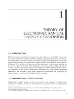
in a form convenient for analysis. These goals may be achieved by starting with two
stationary electric circuits that are magnetically coupled as shown in Figure 1.2-1. The
two coils consist of turns N

1
and N
2
, respectively, and they are wound on a common
core that is generally a ferromagnetic material with permeability large relative to that
of air. The permeability of free space, μ
0
, is 4π × 10
−7
H/m. The permeability of other
materials is expressed as μ = μ
r
μ
0
, where μ
r
is the relative permeability. In the case of
transformer steel, the relative permeability may be as high as 2000–4000.
In general, the flux produced by each coil can be separated into two components.
A leakage component is denoted with an l subscript and a magnetizing component is
denoted by an m subscript. Each of these components is depicted by a single streamline
with the positive direction determined by applying the right-hand rule to the direction
of current flow in the coil. Often, in transformer analysis, i
2
is selected positive out of
the top of coil 2 and a dot placed at that terminal.
The flux linking each coil may be expressed

Φ Φ Φ Φ
1 1 1 2

= + +
l m m
(1.2-1)

Φ Φ Φ Φ
2 2 2 1
= + +
l m m
(1.2-2)
The leakage flux Φ
l1
is produced by current flowing in coil 1, and it links only the turns
of coil 1. Likewise, the leakage flux Φ
l2
is produced by current flowing in coil 2, and
it links only the turns of coil 2. The magnetizing flux Φ
m1
is produced by current flowing
in coil 1, and it links all turns of coils 1 and 2. Similarly, the magnetizing flux Φ
m2
is
produced by current flowing in coil 2, and it also links all turns of coils 1 and 2. With
the selected positive direction of current flow and the manner in that the coils are wound
(Fig. 1.2-1), magnetizing flux produced by positive current in one coil adds to the
Figure 1.2-1. Magnetically coupled circuits.
+
–
n
l
+

–
n
2
φ
ml
φ
m2
φ
l

l
φ
l2
N
l
N
2
i
l
i
2
MAGNETICALLY COUPLED CIRCUITS 3
magnetizing flux produced by positive current in the other coil. In other words, if both
currents are flowing in the same direction, the magnetizing fluxes produced by each
coil are in the same direction, making the total magnetizing flux or the total core flux
the sum of the instantaneous magnitudes of the individual magnetizing fluxes. If the
currents are in opposite directions, the magnetizing fluxes are in opposite directions.
In this case, one coil is said to be magnetizing the core, the other demagnetizing.
Before proceeding, it is appropriate to point out that this is an idealization of the
actual magnetic system. Clearly, all of the leakage flux may not link all the turns of the

coil producing it. Likewise, all of the magnetizing flux of one coil may not link all of
the turns of the other coil. To acknowledge this practical aspect of the magnetic system,
the number of turns is considered to be an equivalent number rather than the actual
number. This fact should cause us little concern since the inductances of the electric
circuit resulting from the magnetic coupling are generally determined from tests.
The voltage equations may be expressed in matrix form as

v ri= +
d
dt
l
(1.2-3)
where r = diag[r
1
r
2
], is a diagonal matrix and

( ) [ ]f
T
f f=
1 2

(1.2-4)
where f represents voltage, current, or flux linkage. The resistances r
1
and r
2
and the
flux linkages λ

1
and λ
2
are related to coils 1 and 2, respectively. Since it is assumed
that Φ
1
links the equivalent turns of coil 1 and Φ
2
links the equivalent turns of coil 2,
the flux linkages may be written

λ
1
= N
1 1
Φ
(1.2-5)

λ
2 2 2
N= Φ
(1.2-6)
where Φ
1
and Φ
2
are given by (1.2-1) and (1.2-2), respectively.
Linear Magnetic System
If saturation is neglected, the system is linear and the fluxes may be expressed as

Φ
l
l
N i
1
1 1
1
=
R
(1.2-7)

Φ
m
m
N i
1
1 1
=
R
(1.2-8)

Φ
l
l
N i
2
2 2
2
=
R

(1.2-9)
4 THEORY OF ELECTROMECHANICAL ENERGY CONVERSION

Φ
m
m
N i
2
2 2
=
R
(1.2-10)
where
R
l1
and
R
l2
are the reluctances of the leakage paths and
R
m
is the reluctance of
the path of the magnetizing fluxes. The product of N times i (ampere-turns) is the
magnetomotive force (MMF), which is determined by the application of Ampere’s law.
The reluctance of the leakage paths is difficult to express and measure. A unique deter-
mination of the inductances associated with the leakage flux is typically either calcu-
lated or approximated from design considerations. The reluctance of the magnetizing
path of the core shown in Figure 1.2-1 may be computed with sufficient accuracy from
the well-known relationship

R =
l
A
µ
(1.2-11)
where l is the mean or equivalent length of the magnetic path, A the cross-section area,
and μ the permeability.
Substituting (1.2-7)–(1.2-10) into (1.2-1) and (1.2-2) yields

Φ
1
1 1
1
1 1 2 2
= + +
N i N i N i
l m m
R R R
(1.2-12)

Φ
2
2 2
2
2 2 1 1
= + +
N i N i N i
l m m
R R R
(1.2-13)

Substituting (1.2-12) and (1.2-13) into (1.2-5) and (1.2-6) yields

λ
1
1
2
1
1
1
2
1
1 2
2
= + +
N
i
N
i
N N
i
l m m
R R R
(1.2-14)

λ
2
2
2
2
2

2
2
2
2 1
1
= + +
N
i
N
i
N N
i
l m m
R R R
(1.2-15)
When the magnetic system is linear, the flux linkages are generally expressed in terms
of inductances and currents. We see that the coefficients of the first two terms on the
right-hand side of (1.2-14) depend upon the turns of coil 1 and the reluctance of the
magnetic system, independent of the existence of coil 2. An analogous statement may
be made regarding (1.2-15). Hence, the self-inductances are defined as

L
N N
L L
l m
l m
11
1
2
1

1
2
1 1
= +
= +
R R
(1.2-16)
MAGNETICALLY COUPLED CIRCUITS 5

L
N N
L L
l m
l m
22
2
2
2
2
2
2 2
= +
= +
R R
(1.2-17)
where L
l1
and L
l2
are the leakage inductances and L

m1
and L
m2
the magnetizing induc-
tances of coils 1 and 2, respectively. From (1.2-16) and (1.2-17), it follows that the
magnetizing inductances may be related as

L
N
L
N
m m2
2
2
1
1
2
=
(1.2-18)
The mutual inductances are defined as the coefficient of the third term of (1.2-14) and
(1.2-15).

L
N N
m
12
1 2
=
R
(1.2-19)

L
N N
m
21
2 1
=
R
(1.2-20)
Obviously, L
12
= L
21
. The mutual inductances may be related to the magnetizing induc-
tances. In particular,

L
N
N
L
N
N
L
m
m
12
2
1
1
1

2
2
=
=
(1.2-21)
The flux linkages may now be written as

l = Li,
(1.2-22)
where

L =






=
+
+










L L
L L
L L
N
N
L
N
N
L L L
l m m
m l m
11 12
21 22
1 1
2
1
1
1
2
2 2 2



(1.2-23)
Although the voltage equations with the inductance matrix L incorporated may be used
for purposes of analysis, it is customary to perform a change of variables that yields
the well-known equivalent T circuit of two magnetically coupled coils. To set the stage
for this derivation, let us express the flux linkages from (1.2-22) as
6 THEORY OF ELECTROMECHANICAL ENERGY CONVERSION

λ
1 1 1 1 1
2
1
2
= + +






L i L i
N
N
i
l m
(1.2-24)

λ
2 2 2 2
1
2
1 2
= + +







L i L
N
N
i i
l m
(1.2-25)
Now we have two choices. We can use a substitute variable for (N
2
/N
1
)i
2
or for (N
1
/N
2
)i
1
.
Let us consider the first of these choices

N i N i
1 2 2 2
′
=
(1.2-26)
whereupon we are using the substitute variable
′
i

2
that, when flowing through coil 1,
produces the same MMF as the actual i
2
flowing through coil 2. This is said to be refer-
ring the current in coil 2 to coil 1, whereupon coil 1 becomes the reference coil. On
the other hand, if we use the second choice, then

N i N i
2 1 1 1
′
=
(1.2-27)
Here,
′
i
1
is the substitute variable that produces the same MMF when flowing through
coil 2 as i
1
does when flowing in coil 1. This change of variables is said to refer the
current of coil 1 to coil 2.
We will derive the equivalent T circuit by referring the current of coil 2 to coil 1;
thus from (1.2-26)

′
=i
N
N
i

2
2
1
2
(1.2-28)
Power is to be unchanged by this substitution of variables. Therefore,

′
=v
N
N
v
2
1
2
2
(1.2-29)
whereupon
v i v i
2 2 2 2
=
′ ′
. Flux linkages, which have the units of volt-second, are related
to the substitute flux linkages in the same way as voltages. In particular,

′
=
λ λ
2
1

2
2
N
N
(1.2-30)
Substituting (1.2-28) into (1.2-24) and (1.2-25) and then multiplying (1.2-25) by N
1
/N
2

to obtain
′
λ
2
, and if we further substitute
( / )N N L
m2
2
1
2
1
for L
m2
into (1.2-25), then

λ
1 1 1 1 1 2
= + +
′
L i L i i

l m
( )
(1.2-31)

′
=
′ ′
+ +
′
λ
2 2 2 1 1 2
L i L i i
l m
( )
(1.2-32)
MAGNETICALLY COUPLED CIRCUITS 7
where

′
=






L
N
N
L

l l2
1
2
2
2
(1.2-33)
The voltage equations become

v r i
d
dt
1 1 1
1
= +
λ
(1.2-34)

′
=
′ ′
+
′
v r i
d
dt
2 2 2
2
λ
(1.2-35)
where

′
=






r
N
N
r
2
1
2
2
2
(1.2-36)
The above voltage equations suggest the T equivalent circuit shown in Figure 1.2-2. It
is apparent that this method may be extended to include any number of coils wound
on the same core.
Figure 1.2-2. Equivalent circuit with coil 1 selected as reference coil.
L
l

2
¢
r
2

¢
i
2
¢
v
2
¢
r
1
i
1
v
1
L
l
1
L
m
1
+
–
+
–
EXAMPLE 1A It is instructive to illustrate the method of deriving an equivalent T
circuit from open- and short-circuit measurements. For this purpose, let us assume that
when coil 2 of the transformer shown in Figure 1.2-1 is open-circuited, the power input
to coil 2 is 12 W when the applied voltage is 110 V (rms) at 60 Hz and the current is
1 A (rms). When coil 2 is short-circuited, the current flowing in coil 1 is 1 A when the
applied voltage is 30 V at 60 Hz. The power during this test is 22 W. If we assume
L L

l l1 2
=
′
, an approximate equivalent T circuit can be determined from these measure-
ments with coil 1 selected as the reference coil.
The power may be expressed as

P V I
1 1 1
=
 
cos
φ
(1A-1)
where

V
and

I
are phasors, and ϕ is the phase angle between

V
1
and

I
1
(power factor
angle). Solving for ϕ during the open-circuit test, we have

8 THEORY OF ELECTROMECHANICAL ENERGY CONVERSION

φ
=
=
×
= °
−
−
cos
cos
.
1
1
1 1
1
83 7
P
V I
 
12
110 1
(1A-2)
With

V
1
as the reference phasor and assuming an inductive circuit where

I

1
lags

V
1
,

Z
V
I
j
=
=
°
− °
= +


1
1
110 0
1 83 7
12 109 3
/
/ .
. Ω
(1A-3)
If we neglect hysteresis (core) losses, then r
1
= 12 Ω. We also know from the above

calculation that X
l1
+ X
m1
= 109.3 Ω.
For the short-circuit test, we will assume that
i i
1 2
= −
′
, since transformers are
designed so that
X r jX
m l1 2 2
>>
′
+
′
. Hence, using (1A-1) again

φ
=
×
= °
−
cos
.
1
22
30 1

42 8
(1A-4)
In this case, the input impedance is
( ) ( )r r j X X
l l1 2 1 2
+
′
+ +
′
. This may be determined as
follows:

Z
j
=
°
− °
= +
30 0
1 42 8
22 20 4
/
/ .
. Ω
(1A-5)
Hence,
′
=
r
2

10 Ω
and, since it is assumed that
X X
l l1 2
=
′
, both are 10.2 Ω. Therefore,
X
m1
= 109.3 − 10.2 = 99.1 Ω. In summary

r L r
L L
m
l l
1 1 2
1 2
12 262 9 10
27 1 27 1
= =
′
=
=
′
=
Ω Ω.
. .
mH
mH mH
Nonlinear Magnetic System

Although the analysis of transformers and electric machines is generally performed
assuming a linear magnetic system, economics dictate that in the practical design of
many of these devices, some saturation occurs and that heating of the magnetic material
exists due to hysteresis loss. The magnetization characteristics of transformer or
machine materials are given in the form of the magnitude of flux density versus
MAGNETICALLY COUPLED CIRCUITS 9
magnitude of field strength (B–H curve) as shown in Figure 1.2-3. If it is assumed that
the magnetic flux is uniform through most of the core, then B is proportional to Φ and
H is proportional to MMF. Hence, a plot of flux versus current is of the same shape as
the B–H curve. A transformer is generally designed so that some saturation occurs
during normal operation. Electric machines are also designed similarly in that a machine
generally operates slightly in the saturated region during normal, rated operating condi-
tions. Since saturation causes coefficients of the differential equations describing the
behavior of an electromagnetic device to be functions of the coil currents, a transient
analysis is difficult without the aid of a computer. Our purpose here is not to set forth
methods of analyzing nonlinear magnetic systems. A method of incorporating the
effects of saturation into a computer representation is of interest.
Formulating the voltage equations of stationary coupled coils appropriate for com-
puter simulation is straightforward, and yet this technique is fundamental to the com-
puter simulation of ac machines. Therefore, it is to our advantage to consider this
method here. For this purpose, let us first write (1.2-31) and (1.2-32) as

λ λ
1 1 1
= +L i
l m
(1.2-37)

′
=

′ ′
+
λ λ
2 2 2
L i
l m
(1.2-38)
where

λ
m m
L i i= +
′
1 1 2
( )
(1.2-39)
Figure 1.2-3. B–H curve for typical silicon steel used in transformers.
1.6
1.2
0.8
0.4
0
B, Wb/m
2
H, A/m
0 200 400 600 800
10 THEORY OF ELECTROMECHANICAL ENERGY CONVERSION
Solving (1.2-37) and (1.2-38) for the currents yields

i

L
l
m1
1
1
1
= −( )
λ λ
(1.2-40)

′
=
′
′
−i
L
l
m2
2
2
1
( )
λ λ
(1.2-41)
If (1.2-40) and (1.2-41) are substituted into the voltage equations (1.2-34) and (1.2-35),
and if we solve the resulting equations for flux linkages, the following equations are
obtained:

λ λ λ
1 1

1
1
1
= + −






∫
v
r
L
dt
l
m
( )
(1.2-42)

′
=
′
+
′
′
−
′







∫
λ λ λ
2 2
2
2
2
v
r
L
dt
l
m
( )
(1.2-43)
Substituting (1.2-40) and (1.2-41) into (1.2-39) yields

λ
λ λ
m a
l l
L
L L
= +
′
′







1
1
2
2
(1.2-44)
where

L
L L L
a
m l l
= + +
′






−
1 1 1
1 1 2
1
(1.2-45)
We now have the equations expressed with λ

1
and
′
λ
2
as state variables. In the computer
simulation, (1.2-42) and (1.2-43) are used to solve for λ
1
and
′
λ
2
, and (1.2-44) is used
to solve for λ
m
. The currents can then be obtained from (1.2-40) and (1.2-41). It is clear
that (1.2-44) could be substituted into (1.2-40)–(1.2-43) and λ
m
eliminated from the
equations, whereupon it would not appear in the computer simulation. However, we
will find λ
m
(the magnetizing flux linkage) an important variable when we include the
effects of saturation.
If the magnetization characteristics (magnetization curve) of the coupled coil are
known, the effects of saturation of the mutual flux path may be incorporated into the
computer simulation. Generally, the magnetization curve can be adequately determined
from a test wherein one of the coils is open-circuited (coil 2, for example) and the input
impedance of coil 1 is determined from measurements as the applied voltage is increased
in magnitude from 0 to say 150% of the rated value. With information obtained from

this type of test, we can plot λ
m
versus
′
+
′
(
)
i i
1 2
as shown in Figure 1.2-4, wherein the
slope of the linear portion of the curve is L
m1
. From Figure 1.2-4, it is clear that in the
region of saturation, we have

λ λ
m m m
L i i f= +
′
−
1 1 2
( ) ( )
(1.2-46)
MAGNETICALLY COUPLED CIRCUITS 11
Figure 1.2-4. Magnetization curve.
λ
i
λ
m

f (λ
m
)
f (i
2
+ )
i
2
¢
L
m1
(i
1
+ )
i
2
¢
i
1
+
i
2
¢
Slope of L
m1
Figure 1.2-5. f(λ
m
) versus λ
m
from Figure 1.2-4.

f (
λ
m
)
λ
m
where f(λ
m
) may be determined from the magnetization curve for each value of λ
m
. In
particular, f(λ
m
) is a function of λ
m
as shown in Figure 1.2-5. Therefore, the effects of
saturation of the mutual flux path may be taken into account by replacing (1.2-39) with
(1.2-46) for λ
m
. Substituting (1.2-40) and (1.2-41) for i
1
and
′
i
2
, respectively, into (1.2-
46) yields the following equation for λ
m
12 THEORY OF ELECTROMECHANICAL ENERGY CONVERSION

λ
λ λ
λ
m a
l l
a
m
m
L
L L
L
L
f= +
′
′






−
1
1
2
2 1
( )
(1.2-47)
Hence, the computer simulation for including saturation involves replacing λ
m

given
by (1.2-44) with (1.2-47), where f(λ
m
) is a generated function of λ
m
determined from
the plot shown in Figure 1.2-5.
1.3.  ELECTROMECHANICAL ENERGY CONVERSION
Although electromechanical devices are used in some manner in a wide variety of
systems, electric machines are by far the most common. It is desirable, however, to
establish methods of analysis that may be applied to all electromechanical devices.
Prior to proceeding, it is helpful to clarify that throughout the book, the words “winding”
and “coil” are used to describe conductor arrangements. To distinguish, a winding
consists of one or more coils connected in series or parallel.
Energy Relationships
Electromechanical systems are comprised of an electrical system, a mechanical system,
and a means whereby the electrical and mechanical systems can interact. Interaction
can take place through any and all electromagnetic and electrostatic fields that are
common to both systems, and energy is transferred from one system to the other as a
result of this interaction. Both electrostatic and electromagnetic coupling fields may
exist simultaneously and the electromechanical system may have any number of electri-
cal and mechanical systems. However, before considering an involved system, it is
helpful to analyze the electromechanical system in a simplified form. An electrome-
chanical system with one electrical system, one mechanical system, and with one
coupling field is depicted in Figure 1.3-1. Electromagnetic radiation is neglected, and
it is assumed that the electrical system operates at a frequency sufficiently low so that
the electrical system may be considered as a lumped parameter system.
Losses occur in all components of the electromechanical system. Heat loss will
occur in the mechanical system due to friction and the electrical system will dissipate
heat due to the resistance of the current-carrying conductors. Eddy current and hyster-

esis losses occur in the ferromagnetic material of all magnetic fields while dielectric
losses occur in all electric fields. If W
E
is the total energy supplied by the electrical
source and W
M
the total energy supplied by the mechanical source, then the energy
distribution could be expressed as

W W W W
E e eL eS
= + +
(1.3-1)

W W W W
M m mL mS
= + +
(1.3-2)
Figure 1.3-1. Block diagram of elementary electromechanical system.
Electrical
system
Mechanical
system
Coupling
field
ELECTROMECHANICAL ENERGY CONVERSION 13
In (1.3-1), W
eS
is the energy stored in the electric or magnetic fields that are not coupled
with the mechanical system. The energy W

eL
is the heat losses associated with the
electrical system. These losses occur due to the resistance of the current-carrying con-
ductors, as well as the energy dissipated from these fields in the form of heat due to
hysteresis, eddy currents, and dielectric losses. The energy W
e
is the energy transferred
to the coupling field by the electrical system. The energies common to the mechanical
system may be defined in a similar manner. In (1.3-2), W
mS
is the energy stored in the
moving member and compliances of the mechanical system, W
mL
is the energy losses
of the mechanical system in the form of heat, and W
m
is the energy transferred to the
coupling field. It is important to note that with the convention adopted, the energy sup-
plied by either source is considered positive. Therefore, W
E
(W
M
) is negative when
energy is supplied to the electrical source (mechanical source).
If W
F
is defined as the total energy transferred to the coupling field, then

W W W
F f fL

= +
(1.3-3)
where W
f
is energy stored in the coupling field and W
fL
is the energy dissipated in the
form of heat due to losses within the coupling field (eddy current, hysteresis, or dielec-
tric losses). The electromechanical system must obey the law of conservation of energy,
thus

W W W W W W W W
f fL E eL eS M mL mS
+ = − − + − −( ) ( )
(1.3-4)
which may be written as

W W W W
f fL e m
+ = +
(1.3-5)
This energy relationship is shown schematically in Figure 1.3-2.
The actual process of converting electrical energy to mechanical energy (or vice
versa) is independent of (1) the loss of energy in either the electrical or the mechanical
systems (W
eL
and W
mL
), (2) the energies stored in the electric or magnetic fields that are
not common to both systems (W

eS
), or (3) the energies stored in the mechanical system
(W
mS
). If the losses of the coupling field are neglected, then the field is conservative
and (1.3-5) becomes [1]

W W W
f e m
= +
(1.3-6)
Figure 1.3-2. Energy balance.
Coupling fieldElectrical system
+ + +
–
–
–
Σ Σ
+
–
–
Σ
–
W
eL
W
E
W
e
W

eS
W
mS
W
m
W
M
W
f
W
fL
W
mL
Mechanical system
14 THEORY OF ELECTROMECHANICAL ENERGY CONVERSION
Examples of elementary electromechanical systems are shown in Figure 1.3-3 and
Figure 1.3-4. The system shown in Figure 1.3-3 has a magnetic coupling field, while
the electromechanical system shown in Figure 1.3-4 employs an electric field as a
means of transferring energy between the electrical and mechanical systems. In these
systems, v is the voltage of the electric source and f is the external mechanical force
applied to the mechanical system. The electromagnetic or electrostatic force is denoted
by f
e
. The resistance of the current-carrying conductors is denoted by r, and l denotes
the inductance of a linear (conservative) electromagnetic system that does not couple
the mechanical system. In the mechanical system, M is the mass of the movable
member, while the linear compliance and damper are represented by a spring constant
K and a damping coefficient D, respectively. The displacement x
0
is the zero force or

equilibrium position of the mechanical system that is the steady-state position of the
mass with f
e
and f equal to zero. A series or shunt capacitance may be included in the
electrical system wherein energy would also be stored in an electric field external to
the electromechanical process.
Figure 1.3-3. Electromechanical system with magnetic field.
φ
K
N
e
f
x
rl
i
v
+
–
+
–
x
0
D
f
f
e
M
Figure 1.3-4. Electromechanical system with electric field.
rl
i

v
+
–
e
f
+
–
K
M
D
+q–q
f
f
e
x
x
0
ELECTROMECHANICAL ENERGY CONVERSION 15
The voltage equation that describes both electrical systems may be written as

v ri l
di
dt
e
f
= + +
(1.3-7)
where e
f
is the voltage drop across the coupling field. The dynamic behavior of the

translational mechanical systems may be expressed by employing Newton’s law of
motion. Thus,

f M
d x
dt
D
dx
dt
K x x f
e
= + + − −
2
2
0
( )
(1.3-8)
The total energy supplied by the electric source is

W vidt
E
=
∫
(1.3-9)
The total energy supplied by the mechanical source is

W fdx
M
=
∫

(1.3-10)
which may also be expressed as

W f
dx
dt
dt
M
=
∫
(1.3-11)
Substituting (1.3-7) into (1.3-9) yields

W r i dt l idi e idt
E f
= + +
∫ ∫ ∫
2
(1.3-12)
The first term on the right-hand side of (1.3-12) represents the energy loss due to the
resistance of the conductors (W
eL
). The second term represents the energy stored in the
linear electromagnetic field external to the coupling field (W
eS
). Therefore, the total
energy transferred to the coupling field from the electrical system is

W e idt
e f

=
∫
(1.3-13)
Similarly, for the mechanical system, we have

W M
d x
dt
dx D
dx
dt
dt K x x dx f dx
M e
= +






+ − −
∫ ∫ ∫ ∫
2
2
2
0
( )
(1.3-14)
Here, the first and third terms on the right-hand side of (1.3-14) represent the energy
stored in the mass and spring, respectively (W

mS
). The second term is the heat loss due
to friction (W
mL
). Thus, the total energy transferred to the coupling field from the
mechanical system with one mechanical input is
16 THEORY OF ELECTROMECHANICAL ENERGY CONVERSION

W f dx
m e
= −
∫
(1.3-15)
It is important to note that a positive force, f
e
, is assumed to be in the same direction
as a positive displacement, x. Substituting (1.3-13) and (1.3-15) into the energy balance
relation, (1.3-6), yields

W e idt f dx
f f e
= −
∫ ∫
(1.3-16)
The equations set forth may be readily extended to include an electromechanical system
with any number of electrical inputs. Thus,

W W W
f ej
j

J
m
= +
=
∑
1
(1.3-17)
wherein J electrical inputs exist. The J here should not be confused with that used later
for the inertia of rotational systems. The total energy supplied to the coupling field from
the electrical inputs is

W e i dt
ej
j
J
fj j
j
J
= =
∑ ∑
∫
=
1 1
(1.3-18)
The total energy supplied to the coupling field from the mechanical input is

W f dx
m e
= −
∫

(1.3-19)
The energy balance equation becomes

W e i dt f dx
f fj j
j
J
e
= −
=
∑
∫ ∫
1
(1.3-20)
In differential form

dW e i dt f dx
f fj j
j
J
e
= −
=
∑
1
(1.3-21)
Energy in Coupling Fields
Before using (1.3-21) to obtain an expression for the electromagnetic force f
e
, it is

necessary to derive an expression for the energy stored in the coupling fields. Once we
have an expression for W
f
, we can take the total derivative to obtain dW
f
that can then
be substituted into (1.3-21). When expressing the energy in the coupling fields, it is
ELECTROMECHANICAL ENERGY CONVERSION 17
convenient to neglect all losses associated with the electric and magnetic fields, where-
upon the fields are assumed to be conservative and the energy stored therein is a func-
tion of the state of the electrical and mechanical variables. Although the effects of the
field losses may be functionally taken into account by appropriately introducing a
resistance in the electric circuit, this refinement is generally not necessary since the
ferromagnetic material is selected and arranged in laminations so as to minimize
the hysteresis and eddy current losses. Moreover, nearly all of the energy stored in the
coupling fields is stored in the air gaps of the electromechanical device. Since air is a
conservative medium, all of the energy stored therein can be returned to the electrical
or mechanical systems. Therefore, the assumption of lossless coupling fields is not as
restrictive as it might first appear.
The energy stored in a conservative field is a function of the state of the system
variables and not the manner in which the variables reached that state. It is convenient
to take advantage of this feature when developing a mathematical expression for the
field energy. In particular, it is convenient to fix mathematically the position of the
mechanical systems associated with the coupling fields and then excite the electrical
systems with the displacements of the mechanical systems held fixed. During the excita-
tion of the electrical systems, W
m
is zero, since dx is zero, even though electromagnetic
or electrostatic forces occur. Therefore, with the displacements held fixed, the energy
stored in the coupling fields during the excitation of the electrical systems is equal to

the energy supplied to the coupling fields by the electrical systems. Thus, with W
m
= 0,
the energy supplied from the electrical system may be expressed from (1.3-20) as

W e i dt
f fj j
j
J
=
=
∑
∫
1
(1.3-22)
It is instructive to consider a single-excited electromagnetic system similar to that
shown in Figure 1.3-3. In this case, e
f
= dλ/dt and (1.3-22) becomes

W id
f
=
∫
λ
(1.3-23)
Here J = 1, however, the subscript is omitted for the sake of brevity. The area to the
left of the λ−i relationship, shown in Figure 1.3-5, for a singly excited electromagnetic
device is the area described by (1.3-23). In Figure 1.3-5, this area represents the energy
stored in the field at the instant when λ = λ

a
and i = i
a
. The λ−i relationship need not
be linear, it need only be single valued, a property that is characteristic to a conservative
or lossless field. Moreover, since the coupling field is conservative, the energy stored
in the field with λ = λ
a
and i = i
a
is independent of the excursion of the electrical and
mechanical variables before reaching this state.
The area to the right of the λ−i curve is called the coenergy, and it is defined as

W di
c
=
∫
λ
(1.3-24)
which may also be written as
18 THEORY OF ELECTROMECHANICAL ENERGY CONVERSION

W i W
c f
= −
λ
(1.3-25)
For multiple electrical inputs, λi in (1.3-25) becomes
λ

j j
j
J
i
=
∑
1
. Although the coenergy
has little or no physical significance, we will find it a convenient quantity for expressing
the electromagnetic force. It should be clear that W
f
= W
c
for a linear magnetic system
where the λ−i plots are straight-line relationships.
The displacement x defines completely the influence of the mechanical system upon
the coupling field; however, since λ and i are related, only one is needed in addition to
x in order to describe the state of the electromechanical system. Therefore, either λ and
x or i and x may be selected as independent variables. If i and x are selected as indepen-
dent variables, it is convenient to express the field energy and the flux linkages as

W W i x
f f
=
( , )
(1.3-26)

λ λ
=
( , )i x

(1.3-27)
With i and x as independent variables, we must express dλ in terms of di before sub-
stituting into (1.3-23). Thus, from (1.3-27)

d i x
i x
i
di
i x
x
dx
λ
λ λ
( , )
( , ) ( , )
=
∂
∂
+
∂
∂
(1.3-28)
Figure 1.3-5. Stored energy and coenergy in a magnetic field of a singly excited electromag-
netic device.
λ
ii
a
W
c
W

f
λ
a
dλ
0
di
ELECTROMECHANICAL ENERGY CONVERSION 19
In the derivation of an expression for the energy stored in the field, dx is set equal to
zero. Hence, in the evaluation of field energy, dλ is equal to the first term on the right-
hand side of (1.3-28). Substituting into (1.3-23) yields

W i x i
i x
i
di
x
d
f
i
( , )
( , ) ( , )
=
∂
∂
=
∂
∂
∫ ∫
λ
ξ

λ ξ
ξ
ξ
0
(1.3-29)
where ξ is the dummy variable of integration. Evaluation of (1.3-29) gives the energy
stored in the field of a singly excited system. The coenergy in terms of i and x may be
evaluated from (1.3-24) as

W i x i x di x d
c
i
( , ) ( , ) ( , )= =
∫ ∫
λ λ ξ ξ
0
(1.3-30)
With λ and x as independent variables

W W x
f f
=
( , )
λ
(1.3-31)

i i x
=
( , ).
λ

(1.3-32)
The field energy may be evaluated from (1.3-23) as

W x i x d i x d
f
( , ) ( , ) ( , )
λ λ λ ξ ξ
λ
= =
∫ ∫
0
(1.3-33)
In order to evaluate the coenergy with λ and x as independent variables, we need to
express di in terms of dλ; thus, from (1.3-32), we obtain

di x( , )
( , ) ( , )
λ
λ
λ
λ
λ
=
∂
∂
+
∂
∂
i x
d

i x
x
dx
(1.3-34)
Since dx = 0 in this evaluation, (1.3-24) becomes

W x
i x
d
i x
d
c
( , )
( , ) ( , )
λ λ
λ
λ
λ ξ
ξ
ξ
ξ
λ
=
∂
∂
=
∂
∂
∫ ∫
0

(1.3-35)
For a linear electromagnetic system, the λ−i plots are straight-line relationships; thus,
for the singly excited system, we have

λ
( , ) ( )i x L x i=
(1.3-36)
or

i x
L x
( , )
( )
λ
λ
=
(1.3-37)
Let us evaluate W
f
(i,x). From (1.3-28), with dx = 0
20 THEORY OF ELECTROMECHANICAL ENERGY CONVERSION

d i x L x di
λ
( , ) ( )
=
(1.3-38)
Hence, from (1.3-29)

W i x L x d L x i

f
i
( , ) ( ) ( )= =
∫
ξ ξ
0
2
1
2
(1.3-39)
It is left to the reader to show that W
f
(λ,x), W
c
(i,x), and W
c
(λ,x) are equal to (1.3-39)
for this magnetically linear system.
The field energy is a state function, and the expression describing the field energy
in terms of system variables is valid regardless of the variations in the system variables.
For example, (1.3-39) expresses the field energy regardless of the variations in L(x) and
i. The fixing of the mechanical system so as to obtain an expression for the field energy
is a mathematical convenience and not a restriction upon the result.
In the case of a multiexcited, electromagnetic system, an expression for the field
energy may be obtained by evaluating the following relation with dx = 0:

W i d
f j j
j
J

=
=
∑
∫
λ
1
(1.3-40)
Because the coupling fields are considered conservative, (1.3-40) may be evaluated
independent of the order in which the flux linkages or currents are brought to their final
values. To illustrate the evaluation of (1.3-40) for a multiexcited system, we will allow
the currents to establish their final states one at a time while all other currents are
mathematically fixed either in their final or unexcited state. This procedure may be
illustrated by considering a doubly excited electric system. An electromechanical
system of this type could be constructed by placing a second coil, supplied from a
second electrical system, on either the stationary or movable member of the system
shown in Figure 1.3-3. In this evaluation, it is convenient to use currents and displace-
ment as the independent variables. Hence, for a doubly excited electric system

W i i x i d i i x i d i i x
f
( , , ) ( , , ) ( , , )
1 2 1 1 1 2 2 2 1 2
= +
[ ]
∫
λ λ
(1.3-41)
In this determination of an expression for W
f
, the mechanical displacement is held

constant (dx = 0); thus (1.3-41) becomes

W i i x i
i i x
i
di
i i x
i
di
f
( , , )
( , , ) ( , , )
1 2 1
1 1 2
1
1
1 1 2
2
2
=
∂
∂
+
∂
∂







∫
λ λ
++
∂
∂
+
∂
∂






i
i i x
i
di
i i x
i
di
2
2 1 2
1
1
2 1 2
2
2
λ λ

( , , ) ( , , )
(1.3-42)
We will evaluate the energy stored in the field by employing (1.3-42) twice. First, we
will mathematically bring the current i
1
to the desired value while holding i
2
at zero.
ELECTROMECHANICAL ENERGY CONVERSION 21
Thus, i
1
is the variable of integration and di
2
= 0. Energy is supplied to the coupling
field from the source connected to coil 1. As the second evaluation of (1.3-42), i
2
is
brought to its desired current while holding i
1
at its desired value. Hence, i
2
is the vari-
able of integration and di
1
= 0. During this time, energy is supplied from both sources
to the coupling field since i
1
dλ
1
is nonzero. The total energy stored in the coupling field

is the sum of the two evaluations. Following this two-step procedure, the evaluation of
(1.3-42) for the total field energy becomes
W i i x i
i i x
i
di i
i i x
i
di i
f
( , , )
( , , ) ( , , )
1 2 1
1 1 2
1
1 1
1 1 2
2
2 2
=
∂
∂
+
∂
∂
+
∂
∫
λ λ λλ
2 1 2

2
2
( , , )i i x
i
di
∂






∫
(1.3-43)
which should be written as
W i i x
i x
d i
i x
d
i
f
i
( , , )
( , , ) ( , , ) (
1 2
1 2
0
1
1 1 2 1

1
=
∂
∂
+
∂
∂
+
∂
∫
ξ
λ ξ
ξ
ξ
λ ξ
ξ
ξ ξ
λ
,, , )
ξ
ξ
ξ
x
d
i
∂







∫
0
2
(1.3-44)
The first integral on the right-hand side of (1.3-43) or (1.3-44) results from the first
step of the evaluation, with i
1
as the variable of integration and with i
2
= 0 and di
2
= 0.
The second integral comes from the second step of the evaluation with i
1
= i
1
, di
1
= 0,
and i
2
as the variable of integration. It is clear that the order of allowing the currents
to reach their final state is irrelevant; that is, as our first step, we could have made i
2

the variable of integration while holding i
1
at zero (di

1
= 0) and then let i
1
become the
variable of integration while holding i
2
at its final value. The result would be the same.
It is also clear that for three electrical inputs, the evaluation procedure would require
three steps, one for each current to be brought mathematically to its final state.
Let us now evaluate the energy stored in a magnetically linear electromechanical
system with two electric inputs. For this, let

λ
1 1 2 11 1 12 2
( , , ) ( ) ( )i i x L x i L x i= +
(1.3-45)

λ
2 1 2 21 1 22 2
( , , ) ( ) ( )i i x L x i L x i= +
(1.3-46)
With that mechanical displacement held constant (dx = 0),

d i i x L x di L x di
λ
1 1 2 11 1 12 2
( , , ) ( ) ( )= +
(1.3-47)

d i i x L x di L x di

λ
2 1 2 12 1 22 2
( , , ) ( ) ( ) .= +
(1.3-48)
It is clear that the coefficients on the right-hand side of (1.3-47) and (1.3-48) are the
partial derivatives. For example, L
11
(x) is the partial derivative of λ
1
(i
1
,i
2
,x) with respect
to i
1
. Appropriate substitution into (1.3-44) gives

W i i x L x d i L x L x d
f
i i
( , , ) ( ) ( ) ( )
1 2 11
0
1 12 22
0
1 2
= + +
[ ]
∫ ∫

ξ ξ ξ ξ
(1.3-49)
which yields
22 THEORY OF ELECTROMECHANICAL ENERGY CONVERSION

W i i x L x i L x i i L x i
f
( , , ) ( ) ( ) ( )
1 2 11 1
2
12 1 2 22 2
2
1
2
1
2
= + +
(1.3-50)
The extension to a linear electromagnetic system with J electrical inputs is straightfor-
ward, whereupon the following expression for the total field energy is obtained as

W i i x L i i
f J pq p q
q
J
p
J
( , , , )
1
11

1
2
… =
==
∑∑
(1.3-51)
It is left to the reader to show that the equivalent of (1.3-22) for a multiexcited elec-
trostatic system is

W e dq
f fj j
j
J
=
=
∑
∫
1
(1.3-52)
Graphical Interpretation of Energy Conversion
Before proceeding to the derivation of expressions for the electromagnetic force, it is
instructive to consider briefly a graphical interpretation of the energy conversion
process. For this purpose, let us again refer to the elementary system shown in Figure
1.3-3, and let us assume that as the movable member moves from x = x
a
to x = x
b
, where
x
b

< x
a
, the λ−i characteristics are given by Figure 1.3-6. Let us further assume that as
the member moves from x
a
to x
b
, the λ−i trajectory moves from point A to point B. It
is clear that the exact trajectory from A to B is determined by the combined dynamics
of the electrical and mechanical systems. Now, the area OACO represents the original
energy stored in field; area OBDO represents the final energy stored in the field. There-
fore, the change in field energy is

∆W OBDO OACO
f
= −area area
(1.3-53)
The change in W
e
, denoted as ΔW
e
, is

∆W id CABDC
e
A
B
= =
∫
λ

λ
λ
area
(1.3-54)
We know that

∆ ∆ ∆W W W
m f e
= −
(1.3-55)
Hence,

∆W OBDO OACO CABDC OABO
m
= − − = − area area area area
(1.3-56)
Here, ΔW
m
is negative; energy has been supplied to the mechanical system from the
coupling field, part of which came from the energy stored in the field and part from the
ELECTROMECHANICAL ENERGY CONVERSION 23
electrical system. If the member is now moved back to x
a
, the λ−i trajectory may be as
shown in Figure 1.3-7. Hence ΔW
m
is still area OABO, but it is now positive, which
means that energy was supplied from the mechanical system to the coupling field, part
of which is stored in the field and part of which is transferred to the electrical system.
The net ΔW

m
for the cycle from A to B back to A is the shaded area shown in Figure
1.3-8. Since ΔW
f
is zero for this cycle

∆ ∆W W
m e
= −
(1.3-57)
For the cycle shown, the net ΔW
e
is negative, thus ΔW
m
is positive; we have generator
action. If the trajectory had been in the counterclockwise direction, the net ΔW
e
would
have been positive and the net ΔW
m
negative, which would represent motor action.
Electromagnetic and Electrostatic Forces
The energy balance relationships given by (1.3-21) may be arranged as

f dx e i dt dW
e fj j
j
J
f
= −

=
∑
1
(1.3-58)
In order to obtain an expression for f
e
, it is necessary to first express W
f
and then take
its total derivative. One is tempted to substitute the integrand of (1.3-22) into (1.3-58)
Figure 1.3-6. Graphical representation of electromechanical energy conversion for λ−i path
A to B.
λ
D
B
x = x
b
x = x
a
A
C
i0
24 THEORY OF ELECTROMECHANICAL ENERGY CONVERSION
Figure 1.3-7. Graphical representation of electromechanical energy conversion for λ−i path
B to A.
λ
B
x = x
b
x = x

a
A
i0
Figure 1.3-8. Graphical representation of electromechanical energy conversion for λ−i path
A to B to A.
λ
B
A
i0
ELECTROMECHANICAL ENERGY CONVERSION 25
for the infinitesimal change of field energy. This procedure is, of course, incorrect, since
the integrand of (1.3-22) was obtained with the mechanical displacement held fixed
(dx = 0), where the total differential of the field energy is required in (1.3-58). In the
following derivation, we will consider multiple electrical inputs; however, we will
consider only one mechanical input, as we noted earlier in (1.3-15). Electromechnical
systems with more than one mechanical input are not common; therefore, the additional
notation necessary to include multiple mechanical inputs is not warranted. Moreover,
the final results of the following derivation may be readily extended to include multiple
mechanical inputs.
The force or torque in any electromechanical system may be evaluated by employ-
ing (1.3-58). In many respects, one gains a much better understanding of the energy
conversion process of a particular system by starting the derivation of the force or
torque expression with (1.3-58) rather than selecting a relationship from a table.
However, for the sake of completeness, derivation of the force equations will be set
forth and tabulated for electromechanical systems with one mechanical input and J
electrical inputs.
For an electromagnetic system, (1.3-58) may be written as

f dx i d dW
e j j

j
J
f
= −
=
∑
λ
1
(1.3-59)
Although we will use (1.3-59), it is helpful to express it in an alternative form. For this
purpose, let us first write (1.3-25) for multiple electrical inputs

λ
j j
j
J
c f
i W W
=
∑
= +
1
(1.3-60)
If we take the total derivative of (1.3-60), we obtain

λ λ
j j
j
J
j j

j
J
c f
di i d dW dW
= =
∑ ∑
+ = +
1 1
(1.3-61)
We realize that when we evaluate the force f
e
we must select the independent variables;
that is, either the flux linkages or the currents and the mechanical displacement x. The
flux linkages and the currents cannot simultaneously be considered independent vari-
ables when evaluating the f
e
. Nevertheless, (1.3-61), wherein both dλ
j
and di
j
appear,
is valid in general, before a selection of independent variables is made to evaluate f
e
.
If we solve (1.3-61) for the total derivative of field energy, dW
f
, and substitute the result
into (1.3-59), we obtain

f dx di dW

e j j
j
J
c
= − +
=
∑
λ
1
(1.3-62)