Chapter 10 DC machines and drives

377
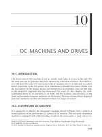
10.1. INTRODUCTION
The direct-current ( dc ) machine is not as widely used today as it was in the past. For
the most part, the dc generator has been replaced by solid-state rectifi ers. Nevertheless,
it is still desirable to devote some time to the dc machine since it is still used as a drive
motor, especially at the low-power level. Numerous textbooks have been written over
the last century on the design, theory, and operation of dc machines. One can add little
to the analytical approach that has been used for years. In this chapter, the well-
established theory of dc machines is set forth, and the dynamic characteristics of the
shunt and permanent-magnet machines are illustrated. The time-domain block diagrams
and state equations are then developed for these two types of motors.
10.2. ELEMENTARY DC MACHINE
It is instructive to discuss the elementary machine shown in Figure 10.2-1 prior to a
formal analysis of the performance of a practical dc machine. The two-pole elementary
machine is equipped with a fi eld winding wound on the stator poles, a rotor coil ( a − a
′
),
Analysis of Electric Machinery and Drive Systems, Third Edition. Paul Krause, Oleg Wasynczuk,
Scott Sudhoff, and Steven Pekarek.
© 2013 Institute of Electrical and Electronics Engineers, Inc. Published 2013 by John Wiley & Sons, Inc.
DC MACHINES AND DRIVES
10
378 DC MACHINES AND DRIVES
and a commutator. The commutator is made up of two semicircular copper segments
mounted on the shaft at the end of the rotor and insulated from one another as well as
from the iron of the rotor. Each terminal of the rotor coil is connected to a copper
segment. Stationary carbon brushes ride upon the copper segments whereby the rotor
coil is connected to a stationary circuit.
The voltage equations for the fi eld winding and rotor coil are

vri

d
dt
fff
f
=+
λ
(10.2-1)

vri
d
dt
aa aaa
aa
−
′
−
′
−
′
=+
λ
(10.2-2)
Figure 10.2-1. Elementary two-pole dc machine.
f
1
f
1
¢
f
2

f
1
f-axis
f
2
¢
f
2
¢
f
2
f
1
¢
¢
Brush
a
a
Insulation
Copper
segment
i
a
v
a
i
a
v
a
i

f
v
f
+
+
–
–
–
q
c
+
ELEMENTARY DC MACHINE 379
where r
f
and r
a
are the resistance of the fi eld winding and armature coil, respectively.
The rotor of a dc machine is commonly referred to as the armature ; rotor and armature
will be used interchangeably. At this point in the analysis, it is suffi cient to express the
fl ux linkages as

λ
fffffaaa
Li Li=+
−
′
(10.2-3)

λ
a a af f aa a a

Li Li
−
′
−
′
=+
(10.2-4)
As a fi rst approximation, the mutual inductance between the fi eld winding and an
armature coil may be expressed as a sinusoidal function of θ
r
as

LL L
af fa r
==−cos
θ
(10.2-5)
where L is a constant. As the rotor revolves, the action of the commutator is to switch
the stationary terminals from one terminal of the rotor coil to the other. For the confi gu-
ration shown in Figure 10.2-1 , this switching or commutation occurs at θ
r
= 0, π , 2 π ,
. . . . At the instant of switching, each brush is in contact with both copper segments,
whereupon the rotor coil is short-circuited. It is desirable to commutate (short-circuit)
the rotor coil at the instant the induced voltage is a minimum. The waveform of the
voltage induced in the open-circuited armature coil during constant-speed operation
with a constant fi eld winding current may be determined by setting
i
aa−
′

= 0
and i
f
equal
to a constant. Substituting (10.2-4) and (10.2-5) into (10.2-2) yields the following
expression for the open-circuit voltage of coil a − a
′
with the fi eld current i
f
a constant:

vLI
aa r f r−
′
=
ωθ
sin
(10.2-6)
where ω
r
= d θ
r
/ dt is the rotor speed. The open-circuit coil voltage
v
aa−
′
is zero at θ
r
= 0,
π , 2 π , . . . , which is the rotor position during commutation. Commutation is illustrated

in Figure 10.2-2 . The open-circuit terminal voltage, ν
a
, corresponding to the rotor posi-
tions denoted as θ
ra
, θ
rb
( θ
rb
= 0), and θ
rc
are indicated. It is important to note that during
one revolution of the rotor, the assumed positive direction of armature current i
a
is down
coil side a and out coil side a
′
for 0 < θ
r
< π . For π < θ
r
< 2 π , positive current is down
coil side a
′
and out of coil side a . Previously, we let positive current fl ow into the
winding denoted without a prime and out the winding denoted with a prime. We will
not be able to adhere to this relationship in the case of the armature windings of a dc
machine since commutation is involved.
The machine shown in Figure 10.2-1 is not a practicable machine. Although it
could be operated as a generator supplying a resistive load, it could not be operated

effectively as a motor supplied from a voltage source owing to the short-circuiting of
the armature coil at each commutation. A practicable dc machine, with the rotor
equipped with an a winding and an A winding, is shown schematically in Figure 10.2-3 .
At the rotor position depicted, coils
aa
44
−
′
and
AA
44
−
′
are being commutated. The
bottom brush short-circuits the
aa
44
−
′
coil while the top brush short-circuits the
AA
44
−
′

coil. Figure 10.2-3 illustrates the instant when the assumed direction of positive current
380 DC MACHINES AND DRIVES
is into the paper in coil sides a
1
, A

1
; a
2
, A
2
; . . . , and out in coil sides
′
a
1
,
′
A
1
;
′
a
2
,
′
A
2
;
. . . It is instructive to follow the path of current through one of the parallel paths from
one brush to the other. For the angular position shown in Figure 10.2-3 , positive cur-
rents enter the top brush and fl ow down the rotor via a
1
and back through
′
a
1

; down a
2

and back through
′
a
2
; down a
3
and back through
′
a
3
to the bottom brush. A parallel
current path exists through
AA
33
−
′
,
AA
22
−
′
, and
AA
11
−
′
. The open-circuit or induced

armature voltage is also shown in Figure 10.2-3 ; however, these idealized waveforms
require additional explanation. As the rotor advances in the counterclockwise direction,
the segment connected to a
1
and A
4
moves from under the top brush, as shown in Figure
10.2-4 . The top brush then rides only on the segment connecting A
3
and
′
A
4
. At the
same time, the bottom brush is riding on the segment connecting a
4
and
′
a
3
. With the
rotor so positioned, current fl ows in A
3
and
′
A
4
and out a
4
and

′
a
3
. In other words, current
fl ows down the coil sides in the upper one half of the rotor and out of the coil sides in
the bottom one half. Let us follow the current fl ow through the parallel paths of the
armature windings shown in Figure 10.2-4 . Current now fl ows through the top brush
into
′
A
4
out A
4
, into a
1
out
′
a
1
, into a
2
, out
′
a
2
, into a
3
out
′
a

3
to the bottom brush. The
Figure 10.2-2. Commutation of the elementary dc machine.
i
a
+
–
a
a
a
¢
a
¢
a
a
¢
q
ra
v
a
i
a
+
–
q
rc
q
rc
q
ra

q
rb
v
a
v
a
i
a
+
–
q
rb
= 0
v
a
ELEMENTARY DC MACHINE 381
Figure 10.2-3. A dc machine with parallel armature windings.
f
1
A
2
A
1
f
1
¢
f
2
f-axis
f

2
¢
a
2
A
3
a
3
A
4
a
4
a
3
-a
3

A
1
a
1
a
1
Rotation
¢
¢
A
2
a
2

¢
¢
A
3
a
3
¢
¢
¢
a
2
-a
2

¢
a
4
-a
4
¢
A
4
-A
4
¢
A
3
-A
3
¢

A
2
-A
2
¢
A
1
-A
1
¢
A
1
-A
1
¢
a
1
-a
1
¢
A
4
a
4
¢
¢
i
a
v
a

v
a
+
–
t
Rotor position
shown above
382 DC MACHINES AND DRIVES
Figure 10.2-4. Same as Figure 10.2-3 , with rotor advanced approximately 22.5°
counterclockwise.
t
f
1
f
1
¢
f
2
f-axis
f
2
¢
A
2
A
1
a
2
a
1

A
3
a
3
A
4
a
4
A
1
a
1
¢
¢
A
2
a
2
¢
¢
A
3
a
3
¢
¢
a
3
-a
3

¢
a
2
-a
2

¢
a
4
-a
4
¢
A
4
-A
4
¢
A
3
-A
3
¢
A
2
-A
2
¢
A
1

-A
1
¢
A
1
-A
1
¢
a
1
-a
1
¢
A
4
a
4
¢
¢
i
a
v
a
v
a
+
–
Rotor position
shown above
p

2pq
r
q
r
w
r
0
ELEMENTARY DC MACHINE 383
parallel path beginning at the top brush is
AA
33
−
′
,
AA
22
−
′
, and
AA
11
−
′
, and
′
−aa
44
to
the bottom brush. The voltage induced in the coils is shown in Figure 10.2-3 and Figure
10.2-4 for the fi rst parallel path described. It is noted that the induced voltage is plotted

only when the coil is in this parallel path.
In Figure 10.2-3 and Figure 10.2-4 , the parallel windings consist of only four coils.
Usually, the number of rotor coils is substantially more than four, thereby reducing the
harmonic content of the open-circuit armature voltage. In this case, the rotor coils may
be approximated as a uniformly distributed winding, as illustrated in Figure 10.2-5 .
Therein, the rotor winding is considered as current sheets that are fi xed in space
due to the action of the commutator and which establish a magnetic axis positioned
orthogonal to the magnetic axis of the fi eld winding. The brushes are shown positioned
on the current sheet for the purpose of depicting commutation. The small angular
Figure 10.2-5. Idealized dc machine with uniformly distributed rotor winding.
Current into
paper
2g
Short-circuited
coils
Rotation
a-axis –
Magnetic axis
of equivalent
armature winding
f-axis
Current out
of paper
i
a
i
a
i
f
v

f
N
f
v
a
+
_
v
a
r
a
r
f
+
_
384 DC MACHINES AND DRIVES
displacement, denoted by 2 γ , designates the region of commutation wherein the coils
are short-circuited. However, commutation cannot be visualized from Figure 10.2-5 ;
one must refer to Figure 10.2-3 and Figure 10.2-4 .
In our discussion of commutation, it was assumed that the armature current was
zero. With this constraint, the sinusoidal voltage induced in each armature coil crosses
through zero when the coil is orthogonal to the fi eld fl ux. Hence, the commutator was
arranged so that the commutation would occur when an armature coil was orthogonal
to fi eld fl ux. When current fl ows in the armature winding, the fl ux established therefrom
is in an axis orthogonal to the fi eld fl ux. Thus, a voltage will be induced in the armature
coil that is being commutated as a result of “cutting” the fl ux established by the current
fl owing in the other armature coils. Arcing at the brushes will occur, and the brushes
and copper segments may be damaged with even a relatively small armature current.
Although the design of dc machines is not a subject of this text, it is important to
mention that brush arcing may be substantially reduced by mechanically shifting the

position of the brushes as a function of armature current or by means of interpoles.
Interpoles or commutating poles are small stator poles placed over the coil sides of the
winding being commutated, midway between the main poles of large horsepower
machines. The action of the interpole is to oppose the fl ux produced by the armature
current in the region of the short-circuited coil. Since the fl ux produced in this region
is a function of the armature current, it is desirable to make the fl ux produced by the
interpole a function of the armature current. This is accomplished by winding the
interpole with a few turns of the conductor carrying the armature current. Electrically,
the interpole winding is between the brush and the terminal. It may be approximated
in the voltage equations by increasing slightly the armature resistance and inductance
( r
a
and L
AA
).
10.3. VOLTAGE AND TORQUE EQUATIONS
Although rigorous derivation of the voltage and torque equations is possible, it is rather
lengthy and little is gained since these relationships may be deduced. The armature
coils revolve in a magnetic fi eld established by a current fl owing in the fi eld winding.
We have established that voltage is induced in these coils by virtue of this rotation.
However, the action of the commutator causes the armature coils to appear as a station-
ary winding with its magnetic axis orthogonal to the magnetic axis of the fi eld winding.
Consequently, voltages are not induced in one winding due to the time rate of change
of the current fl owing in the other (transformer action). Mindful of these conditions,
we can write the fi eld and armature voltage equations in matrix form as

v
v
rpL
LrpL

i
i
f
a
fFF
rAF a AA
f
a
⎡
⎣
⎢
⎤
⎦
⎥
=
+
+
⎡
⎣
⎢
⎤
⎦
⎥
⎡
⎣
⎢
⎤
⎦
⎥
0

ω
(10.3-1)
where L
FF
and L
AA
are the self-inductances of the fi eld and armature windings, respec-
tively, and p is the short-hand notation for the operator d/dt . The rotor speed is denoted
as ω
r
, and L
AF
is the mutual inductance between the fi eld and the rotating armature
VOLTAGE AND TORQUE EQUATIONS 385
coils. The above equation suggests the equivalent circuit shown in Figure 10.3-1 . The
voltage induced in the armature circuit, ω
r
L
AF
i
f
, is commonly referred to as the counter
or back emf. It also represents the open-circuit armature voltage.
A substitute variable often used is

kLi
vAFf
=
(10.3-2)
We will fi nd this substitute variable is particularly convenient and frequently used.

Even though a permanent-magnet dc machine has no fi eld circuit, the constant
fi eld fl ux produced by the permanent magnet is analogous to a dc machine with a
constant k
v
. For a dc machine with a fi eld winding, the electromagnetic torque can be
expressed

TLii
eAFfa
=
(10.3-3)
Here again the variable k
v
is often substituted for L
AF
i
f
. In some instances, k
v
is multi-
plied by a factor less than unity when substituted into (10.3-5) so as to approximate
the effects of rotational losses. It is interesting that the fi eld winding produces a station-
ary MMF and, owing to commutation, the armature winding also produces a stationary
MMF that is displaced (1/2) π electrical degrees from the MMF produced by the fi eld
winding. It follows then that the interaction of these two MMF ’ s produces the electro-
magnetic torque.
The torque and rotor speed are related by

TJ
d

dt
BT
e
r
mr L
=++
ω
ω
(10.3-4)
where J is the inertia of the rotor and, in some cases, the connected mechanical load.
The units of the inertia are kg·m
2
or J·s
2
. A positive electromagnetic torque T
e
acts to
turn the rotor in the direction of increasing θ
r
. The load torque T
L
is positive for a
torque, on the shaft of the rotor, which opposes a positive electromagnetic torque T
e
.
The constant B
m
is a damping coeffi cient associated with the mechanical rotational
system of the machine. It has the units of N·m·s and it is generally small and often
neglected.

Figure 10.3-1. Equivalent circuit of dc machine.
+
–
––
++
r
f
r
a
i
f
i
a
v
a
v
f
L
FF
L
AF
w
r
i
f
L
AA
386 DC MACHINES AND DRIVES
10.4. BASIC TYPES OF DC MACHINES
The fi eld and armature windings may be excited from separate sources or from the

same source with the windings connected differently to form the basic types of dc
machines, such as the shunt-connected, the series-connected, and the compound-
connected dc machines. The equivalent circuits for each of these machines are given
in this section along with an analysis and discussion of their steady-state operating
characteristics.
Separate Winding Excitation
When the fi eld and armature windings are supplied from separate voltage sources, the
device may operate as either a motor or a generator; it is a motor if it is driving a torque
load and a generator if it is being driven by some type of prime mover. The equivalent
circuit for this type of machine is shown in Figure 10.4-1 . It differs from that shown
in Figure 10.3-1 in that external resistance r
fx
is connected in series with the fi eld
winding. This resistance, which is often referred to as a fi eld rheostat , is used to adjust
the fi eld current if the fi eld voltage is supplied from a constant source.
The voltage equations that describe the steady-state performance of this device
may be written directly from (10.3-1) by setting the operator p to zero ( p = d/dt ),
whereupon

VRI
fff
=
(10.4-1)

VrI LI
aaa rAFf
=+
ω
(10.4-2)
where R

f
= r
fx
+ r
f
and capital letters are used to denote steady-state voltages and cur-
rents. We know from the torque relationship given by (10.3-6) that during steady-state
operation T
e
= T
L
if B
m
is assumed to be zero. Analysis of steady-state performance is
straightforward.
A permanent-magnet dc machine fi ts into this class of dc machines. As we have
mentioned, the fi eld fl ux is established in these devices by a permanent magnet. The
voltage equation for the fi eld winding is eliminated, and L
AF
i
f
is replaced by a constant
k
v
, which can be measured if it is not given by the manufacturer. Most small, hand-held,
fractional-horsepower dc motors are of this type, and speed control is achieved by
controlling the amplitude of the applied armature voltage.
Figure 10.4-1. Equivalent circuit for separate fi eld and armature excitation.
+
–

–
–
++
r
fx
r
f
r
a
i
f
i
a
v
a
v
f
L
FF
L
AF
w
r
i
f
L
AA
BASIC TYPES OF DC MACHINES 387
Shunt-Connected dc Machine
The fi eld and armature windings may be connected as shown schematically in Figure

10.4-2 . With this connection, the machine may operate either as a motor or a generator.
Since the fi eld winding is connected between the armature terminals, V
a
= V
f
. This
winding arrangement is commonly referred to as a shunt-connected dc machine or
simply a shunt machine. During steady-state operation, the armature circuit voltage
equation is (10.4-2) and, for the fi eld circuit,

VIR
aff
=
(10.4-3)
The total current I
t
is

III
tfa
=+
(10.4-4)
Solving (10.4-2) for I
a
and (10.4-3) for I
f
and substituting the results in (10.3-3) yields
the following expression for the steady-state electromagnetic torque, positive for motor
action, for this type of dc machine:

T
LV
rR
L
R
e
AF a
af
AF
f
r
=−
⎛
⎝
⎜
⎞
⎠
⎟
2
1
ω
(10.4-5)
The shunt-connected dc machine may operate as either a motor or a generator when
connected to a dc source. It may also operate as an isolated self-excited generator, sup-
plying an electric load, such as a dc motor or a static load. When the shunt machine is
operated from a constant-voltage source, the steady-state operating characteristics are
those shown in Figure 10.4-3 . Several features of these characteristics warrant discus-
sion. At stall ( ω
r
= 0), the steady-state armature current I

a
is limited only by the armature
resistance. In the case of small, permanent-magnet motors, the armature resistance is
quite large so that the starting armature current, which results when rated voltage is
applied, is generally not damaging. However, larger-horsepower machines are designed
with a small armature resistance. Therefore, an excessively high armature current will
occur during the starting period if rated voltage is applied to the armature terminals.
Figure 10.4-2. Equivalent circuit of a shunt-connected dc machine.
+
–
––
+
+
r
fx
r
f
r
a
i
f
i
a
i
t
v
a
v
f
L

FF
L
AF
w
r
i
f
L
AA
388 DC MACHINES AND DRIVES
To prevent high starting current, resistance may be inserted into the armature circuit at
stall and decreased either manually or automatically to zero as the machine accelerates
to normal operating speed. When silicon-controlled rectifi er s ( SCR ’ s) or thyristors are
used to convert an ac source voltage to dc to supply the dc machine, they may be
controlled to provide a reduced voltage during the starting period, thereby preventing
a high starting current and eliminating the need to insert resistance into the armature
circuit. Other features of the shunt machine with a small armature resistance are the
steep torque-versus-speed characteristics. In other words, the speed of the shunt machine
does not change appreciably as the load torque is varied from zero to rated.
Series-Connected dc Machine
When the fi eld is connected in series with the armature circuit, as shown in Figure
10.4-4 , the machine is referred to as a series-connected dc machine or a series machine.
It is convenient to add the subscript s to denote quantities associated with the series
fi eld. It is important to mention the physical difference between the fi eld winding of
a shunt machine and that of a series machine. If the fi eld winding is to be a shunt-
connected winding, it is wound with a large number of turns of small-diameter wire,
Figure 10.4-3. Steady-state operating characteristics of a shunt-connected dc machine with
constant source voltage.
V
a

V
a
R
f
r
a
+
r
a
R
f
L
AF
V
a
L
AF
I
t
T
e
V
a
R
f
R
f
w
r
2

BASIC TYPES OF DC MACHINES 389
making the resistance of the fi eld winding quite large. However, since the series-
connected fi eld winding is in series with the armature, it is designed so as to minimize
the voltage drop across it. Thus, the winding is wound with a few turns of low-
resistance wire.
Although the series machine does not have wide application, a series fi eld is often
used in conjunction with a shunt fi eld to form a compound-connected dc machine,
which is more common. In the case of a series machine (Fig. 10.4-4 ),

vv v
tfsa
=+
(10.4-6)

ii
afs
=
(10.4-7)
where v
fs
and i
fs
denote the voltage and current associated with the series fi eld. The
subscript s is added to avoid confusion with the shunt fi eld when both fi elds are used
in a compound machine.
If the constraints given by (10.4-6) and (10.4-7) are substituted into the armature
voltage equation, the steady-state performance of the series-connected dc machine may
be described by

VrrL I

t a fs AFs r a
=++()
ω
(10.4-8)
From (10.3-5) ,

TLI
LV
rr L
e AFs a
AFs t
a fs AFs r
=
=
++
2
2
2
()
ω
(10.4-9)
The steady-state torque–speed characteristic for a typical series machine is shown in
Figure 10.4-5 . The stall torque is quite high since it is proportional to the square of the
armature current for a linear magnetic system. However, saturation of the magnetic
system due to large armature currents will cause the torque to be less than that calcu-
lated from (10.4-9) . At high rotor speeds, the torque decreases less rapidly with increas-
ing speed. In fact, if the load torque is small, the series motor may accelerate to speeds
large enough to cause damage to the machine. Consequently, the series motor is used
Figure 10.4-4. Equivalent circuit for a series-connected dc machine.
+

––
–
–
++
+
r
fs
r
a
i
fs
i
a
v
a
v
t
v
fs
L
FF
L
AF
w
r
i
fs
L
AA
390 DC MACHINES AND DRIVES

in applications such as traction motors for trains and buses or in hoists and cranes where
high starting torque is required and an appreciable load torque exists under normal
operation.
Compound-Connected dc Machine
A compound-connected or compound dc machine, which is equipped with both a shunt
and a series fi eld winding, is illustrated in Figure 10.4-6 . In most compound machines,
the shunt fi eld dominates the operating characteristics while the series fi eld, which
consists of a few turns of low-resistance wire, has a secondary infl uence. It may be
Figure 10.4-6. Equivalent circuit of a compound dc machine.
+
–
–––
+++
r
fs
r
fx
r
f
r
a
i
fs
i
f
v
f
i
a
i

t
v
t
v
a
v
fs
+
–
L
FFs
L
FF
L
AF
w
r
i
f
± L
AF
w
r
i
fs
L
AA
A
B
Figure 10.4-5. Steady-state torque–speed characteristics of a series-connected dc machine.

T
e
(r
a
+ r
fs
)
2
V
t
2
L
AFs
0
w
r
BASIC TYPES OF DC MACHINES 391
connected so as to aid or oppose the fl ux produced by the shunt fi eld. If the compound
machine is to be used as a generator, the series fi eld is connected so to aid the shunt fi eld
(cumulative compounding). Depending upon the strength of the series fi eld, this type of
connection can produce a “fl at” terminal-voltage-versus-load-current characteristic,
whereupon a near-constant terminal voltage is achieved from no load to full load. In this
case, the machine is said to be “fl at compounded.” An “overcompounded” machine
occurs when the strength of the series fi eld causes the terminal voltage at full load to be
larger than at no load. The meaning of the “undercompound” machine is obvious. In the
case of compound dc motors, the series fi eld is often connected to oppose the fl ux pro-
duced by the shunt fi eld (differential compounding). If properly designed, this type of
connection can provide a near-constant speed from no-load to full-load torque.
The voltage equations for a compound dc machine may be written as

v
v
RpL pL
LpL LrpLrpL
f
t
fFF FS
r AF FS r AFs fs FFs a AA
⎡
⎣
⎢
⎤
⎦
⎥
=
+±
±±++ +
0
ωω
⎡⎡
⎣
⎢
⎤
⎦
⎥
⎡
⎣
⎢
⎢
⎢

⎤
⎦
⎥
⎥
⎥
i
i
i
f
fs
a
(10.4-10)
where L
FS
is the mutual inductance between the shunt and the series fi elds. The plus
and minus signs are used so that either a cumulative or a differential connection may
be described.
The shunt fi eld may be connected ahead of the series fi eld (long-shunt connection)
or behind the series fi eld (short-shunt connection), as shown by A and B , respectively,
in Figure 10.4-6 . The long-shunt connection is commonly used. In this case

vv v v
tffsa
==+
(10.4-11)

iii
tffs
=+
(10.4-12)

where

ii
fs a
=
(10.4-13)
The steady-state performance of a long shunt-connected compound machine may be
described by the following equations:

V
rr L
LR
I
t
a fs AFs r
AF f r
a
=
+±
−
⎡
⎣
⎢
⎤
⎦
⎥
ω
ω
1( / )
(10.4-14)

The torque for the long-shunt connection may be obtained by employing (10.3-3) for
each fi eld winding. In particular,

TLIILII
LV L R
Rr r L
e AFfa AFfsa
AF t AF f r
f a fs AFs r
=±
=
−
+±
±
2
1[( /)]
()
ω
ω
LLV L R
rr L
AFs t AF f r
a fs AFs r
22
2
1[( /)]
()
−
+±
ω

ω
(10.4-15)
392 DC MACHINES AND DRIVES
EXAMPLE 10A A permanent-magnet dc motor is rated at 6 V with the following
parameters: r
a
= 7 Ω , L
AA
= 120 mH, k
T
= 2 oz·in/A, J = 150 μ oz·in·s
2
. According to
the motor information sheet, the no-load speed is approximately 3350 r/min, and the
no-load armature current is approximately 0.15 A. Let us attempt to interpret this
information.
First, let us convert k
T
and J to units that we have been using in this book. In this
regard, we will convert the inertia to kg·m
2
, which is the same as N·m·s
2
. To do this,
we must convert ounces to newtons and inches to meters (Appendix A). Thus,

J =
×
=× ⋅
−

−
150 10
3 6 39 37
106 10
6
62
(.)( . )
.kgm
(10A-1)
We have not seen k
T
before. It is the torque constant and, if expressed in the appropriate
units, it is numerically equal to k
v
. When k
v
is used in the expression for T
e
( T
e
= k
v
i
a
),
it is often referred to as the torque constant and denoted as k
T
. When used in the voltage
equation, it is always denoted as k
v

. Now we must convert ounce·in into newton·meter,
whereupon k
T
equals our k
v
; hence,

k
v
==×⋅=×⋅
−−
2
16 0 225 39 37
1 41 10 1 41 10
22
()(. )(.)
N m/A V s/rad
(10A-2)
What do we do about the no-load armature current? What does it represent? Well,
probably it is a measure of the friction and windage losses. We could neglect it, but we
will not. Instead, let us include it as B
m
. First, however, we must calculate the no-load
speed. We can solve for the no-load rotor speed from the steady-state armature voltage
equation for the shunt machine, (10.4-2) , with L
AF
i
f
replaced by k
v

:

ω
π
r
aaa
v
VrI
k
=
−
=
−
×
=
=
−
67015
141 10
351 1
2
()(. )
.
. rad/s
(351.1)(60)
2
== 3353 r/min
(10A-3)
Now at this no-load speed,

Tki
eva
== × = × ⋅
−−
(. )(. ) .141 10 015 212 10
23
Nm
(10A-4)
Since T
L
and J ( d ω
r
/ dt ) are zero for this steady-state no-load condition, (10.3-4) tells us
that (10A-4) is equal to B
m
ω
r
; hence,

B
m
r
=
×
=
×
=× ⋅⋅
−−
−
2 12 10 2 12 10

351 1
604 10
33
6

.
.
ω
Nms
(10A-5)
BASIC TYPES OF DC MACHINES 393
EXAMPLE 10B The permanent-magnet dc machine described in Example 10A is
operating with rated applied armature voltage and load torque T
L
of 0.5 oz·in. Our task
is to determine the effi ciency where percent eff = (power output/power input) 100.
First let us convert ounce·in into newton·meter:

T
L
==×⋅
−
05
16 0 225 39 37
353 10
3
.
()(. )(.)
.Nm
(10B-1)

In Example 10A, we determined k
v
to be 1.41 × 10
− 2
V s/rad and B
m
to be 6.04 × 10
− 6
N·m·s.
During steady-state operation, (10.3-6) becomes

TB T
emrL
=+
ω
(10B-2)
From (10.3-5) , with L
AF
i
f
replaced by k
v
, the steady-state electromagnetic torque is

TkI
eva
=
(10B-3)
Substituting (10B-3) into (10B-2) and solving for ω
r

yields

ω
r
v
m
a
m
L
k
B
I
B
T=−
1
(10B-4)
From (10.4-2) with L
AF
i
f
= k
v
,

VrIk
aaavr
=+
ω
(10B-5)
Substituting (10B-4) into (10B-5) and solving for I

a
yields

I
VkBT
rkB
a
avmL
avm
=
+
+
=
+× ×
−−
(/ )
(/ )
[( . ) / ( . )]( .
2
26
6 1 41 10 6 04 10 3 53310
7 1 41 10 6 04 10
0 357
3
22 6
×
+× ×
=
−
−−

)
(. ) /(. )
.A (10B-6)
From (10B-4) ,

ω
r
=
×
×
−
×
×
=
−
−−
−
141 10
604 10
0 357
1
604 10
353 10
249
2
66
3
.
.
.

.
(. )
rad/s
(10B-7)
The power input is

PVI
aain
W== =()(. ) .6 0 357 2 14
(10B-8)
The power output is
394 DC MACHINES AND DRIVES

PT
Lrout
W==× =
−
ω
(. )( ) .353 10 249 08
3
(10B-9)
The effi ciency is

η
=
==
P
P
out
in

%
100
088
214
100 41 1
.
.
.
(10B-10)
The low effi ciency is characteristic of low-power dc motors due to the relatively large
armature resistance. In this regard, it is interesting to determine the losses due to i
2
r ,
friction, and windage.

PrI
ir
aa
2
22
7 0 357 0 89== =()(. ) . W
(10B-11)

PB
fw m r r
==× =
−
()(. )().
ωω
604 10 249 037

62
W
(10B-12)
Let us check our work:

PPPP
ir
fwin out
W=++= + + =
2
089 037 088 214
(10B-13)
which is equal to (10B-8) .
10.5. TIME-DOMAIN BLOCK DIAGRAMS AND STATE EQUATIONS
Although the analysis of control systems is not our intent, it is worthwhile to set the
stage for this type of analysis by means of a “fi rst look” at time-domain block diagrams
and state equations. In this section, we will consider only the shunt and permanent-
magnet dc machines. The series and compound machines are treated in problems at the
end of the chapter.
Shunt-Connected dc Machine
Block diagrams, which portray the interconnection of the system equations, are used
extensively in control system analysis and design. Although block diagrams are gener-
ally depicted by using the Laplace operator, we shall work with the time-domain equa-
tions for now, using the p operator to denote differentiation with respect to time and
the operator 1/ p to denote integration
Arranging the equations of a shunt machine into a block diagram representation is
straightforward. The fi eld and armature voltage equations, (10.3-1) , and the relationship
between torque and rotor speed, (10.3-4) , may be written as

vR pi

ff ff
=+()1
τ
(10.5-1)

vr pi Li
aa aa rAFf
=+ +()1
τω
(10.5-2)
TIME-DOMAIN BLOCK DIAGRAMS AND STATE EQUATIONS 395

TT B Jp
eL m r
−= +()
ω
(10.5-3)
where the fi eld time constant τ
f
= L
FF
/R
f
and the armature time constant τ
a
= L
AA
/ r
a
.

Here, again, p denotes d/dt and 1/ p will denote integration. Solving (10.5-1) for i
f
,
(10.5-2) for i
a
, and (10.5-3) for ω
r
yields

i
R
p
v
f
f
f
f
=
+
1
1
/
τ
(10.5-4)

i
r
p
vLi
a

a
a
arAFf
=
+
−
1
1
/
()
τ
ω
(10.5-5)

ω
r
m
eL
Jp B
TT=
+
−
1
()
(10.5-6)
The time-domain block diagram portraying (10.5-4) through (10.5-6) with T
e
= L
AF
i

f
i
a

is shown in Figure 10.5-1 . This diagram consists of a set of linear blocks, wherein the
relationship between the input and corresponding output variable is depicted in transfer
function form and a pair of multipliers that represent nonlinear blocks.
The state equations of a system represent the formulation of the state variables into
a matrix form convenient for computer implementation, particularly for linear systems.
The state variables of a system are defi ned as a minimal set of variables such that
knowledge of these variables at any initial time t
0
plus information on the input excita-
tion subsequently applied is suffi cient to determine the state of the system at any time
t > t
0
[1] . In the case of dc machines, the fi eld current i
f
, the armature current i
a
, the
rotor speed ω
r
, and the rotor position θ
r
are chosen as state variables. The rotor position
θ
r
can be established from ω
r

by

ω
θ
r
r
d
dt
=
(10.5-7)
Figure 10.5-1. Time-domain block diagram of a shunt-connected dc machine.
v
f
i
f
i
a
1/R
f
L
AF
T
L
T
e
t
f
p+1
1
Jp+B

m
1/r
a
t
a
p+1
w
r
L
AF
i
f
S
S
v
a
+
–
+
–
w
r
396 DC MACHINES AND DRIVES
Since θ
r
is considered a state variable only when the shaft position is a controlled vari-
able, we will omit θ
r
from consideration in this development.
The formulation of the state equations for the shunt machine can be readily

achieved by straightforward manipulation of the fi eld and armature voltage equations
given by (10.3-1) and the equation relating torque and rotor speed given by (10.3-4) .
In particular, solving the fi eld voltage equation (10.3-1) for di
f
/ dt yields

di
dt
R
L
i
L
v
ff
FF
f
FF
f
=− +
1
(10.5-8)
Solving the armature voltage equation, (10.3-1) , for di
a
/ dt yields

di
dt
r
L
i

L
L
i
L
v
aa
AA
a
AF
AA
fr
AA
a
=− − +
ω
1
(10.5-9)
If we wish, we could use k
v
for L
AF
i
f
; however, we shall not make this substitution.
Solving (10.3-4) for d ω
r
/ dt with T
e
= L
AF

i
f
i
a
yields

d
dt
B
J
L
J
ii
J
T
rm
r
AF
fa L
ω
ω
=− + −
1
(10.5-10)
All we have done here is to solve the equations for the highest derivative of the state
variables while substituting (10.3-3) for T
e
into (10.3-4) . Now let us write the state
equations in matrix (or vector matrix) form as

p
i
i
R
L
r
L
B
J
f
a
r
f
FF
a
AA
m
ω
⎡
⎣
⎢
⎢
⎢
⎤
⎦
⎥
⎥
⎥
=
−

−
−
⎡
⎣
⎢
⎢
⎢
⎢
⎢
⎢
⎢
⎤
⎦
⎥
⎥
⎥
⎥
⎥
⎥
⎥
00
00
00
ii
i
L
L
i
L
J

ii
f
a
r
AF
AA
fr
AF
fa
ω
ω
⎡
⎣
⎢
⎢
⎢
⎤
⎦
⎥
⎥
⎥
+−
⎡
⎣
⎢
⎢
⎢
⎢
⎢
⎢

⎢
⎤
⎦
⎥
⎥
⎥
⎥
⎥
⎥
⎥
+
0
1
LL
L
J
v
v
T
FF
AA
f
a
L
00
0
1
0
00
1

−
⎡
⎣
⎢
⎢
⎢
⎢
⎢
⎢
⎢
⎤
⎦
⎥
⎥
⎥
⎥
⎥
⎥
⎥
⎡
⎣
⎢
⎢
⎢
⎤
⎦
⎥
⎥
⎥

(10.5-11)
where p is the operator d/dt . Equation (10.5-11) is the state equation(s); however, note
that the second term (vector) on the right-hand side contains the products of state vari-
ables causing the system to be nonlinear.
Permanent-Magnet dc Machine
As we have mentioned previously, the equations that describe the operation of a
permanent-magnet dc machine are identical to those of a shunt-connected dc machine
with the fi eld current constant. Thus, the work in this section applies to both. For the
permanent-magnet machine, L
AF
i
f
is replaced by k
v
, which is a constant determined by
TIME-DOMAIN BLOCK DIAGRAMS AND STATE EQUATIONS 397
the strength of the magnet, the reluctance of the iron and air gap, and the number of
turns of the armature winding. The time-domain block diagram may be developed for
the permanent-magnet machine by using (10.5-2) and (10.5-3) , with k
v
substituted for
L
AF
i
f
. The time-domain block diagram for a permanent-magnet dc machine is shown in
Figure 10.5-2 .
Since k
v
is constant, the state variables are now i

a
and ω
r
. From (10.5-9) , for a
permanent-magnet machine,

di
dt
r
L
i
k
LL
v
aa
AA
a
v
AA
r
AA
a
=− − +
ω
1
(10.5-12)
From (10.5-10) ,

d
dt

B
J
k
J
i
J
T
rm
r
v
aL
ω
ω
=− + −
1
(10.5-13)
The system is described by a set of linear differential equations. In matrix form, the
state equations become

p
i
r
L
k
L
k
J
B
J
i

L
a
r
a
AA
v
AA
vm
a
r
AA
ωω
⎡
⎣
⎢
⎤
⎦
⎥
=
−−
−
⎡
⎣
⎢
⎢
⎢
⎢
⎤
⎦
⎥

⎥
⎥
⎥
⎡
⎣
⎢
⎤
⎦
⎥
+
1
00
0
1
−
⎡
⎣
⎢
⎢
⎢
⎢
⎤
⎦
⎥
⎥
⎥
⎥
⎡
⎣
⎢

⎤
⎦
⎥
J
v
T
a
L
(10.5-14)
The form in which the state equations are expressed in (10.5-14) is called the
fundamental form. In particular, the previous matrix equation may be expressed sym-
bolically as

pxAxBu=+
(10.5-15)
which is called the fundamental form, where p is the operator d/dt , x is the state vector
(column matrix of state variables), and u is the input vector (column matrix of inputs
to the system). We see that (10.5-14) and (10.5-15) are identical in form. Methods of
Figure 10.5-2. Time-domain block diagram of a permanent-magnet dc machine.
v
a
i
a
k
v
k
v
T
e
T

L
k
v
w
r
1/r
a
t
a
p+1
SS
+
–
+
–
1
Jp+B
m
w
r
398 DC MACHINES AND DRIVES
solving equations of the fundamental form given by (10.5-15) are well known. Conse-
quently, it is used extensively in control system analysis [1] .
10.6. SOLID-STATE CONVERTERS FOR DC DRIVE SYSTEMS
Numerous types of ac/dc and dc/dc converters are used in variable-speed drive systems
to supply an adjustable dc voltage to the dc drive machine. In the case of ac/dc convert-
ers, half-wave, semi-, full and dual converters are used depending upon the amount of
power being handled and the application requirements; such as fast response time,
regeneration, and reversible or nonreversible drives. In the case of dc/dc converters,
one-, two-, and four-quadrant converters are common. Obviously, we cannot treat all

types of converters and all important applications; instead, it is our objective in this
section to present the widely used converters and to set the stage for the following
sections wherein the analysis and performance of several common dc drive systems are
set forth.
Single-Phase ac / dc Converters
Several types of single-phase phase-controlled ac/dc converters are shown in Figure
10.6-1 . Therein, the converters consist of SCRs and diodes. The dc machine is illus-
trated in abbreviated form without showing the fi eld winding and the resistance and
inductance of the armature winding. The dc machines that are generally used with ac/
dc converters are the permanent magnet, shunt, or series machines. Half-wave, semi-,
full, and dual converters are shown in Figure 10.6-1 .
The half-wave converter yields discontinuous armature current in all modes of
operation, and only positive current fl ows on the ac side of the converter. Analysis of the
operation of a dc drive with discontinuous armature current is quite involved [2] and not
considered. The other converters shown in Figure 10.6-1 can operate with either a con-
tinuous or discontinuous armature current. The half-wave and the semi-converters allow
a positive dc voltage and unidirectional armature current; however, the semi-converter
may be equipped with a diode connected across the terminals of the machine (free-
wheeling diode) to dissipate energy stored in the armature inductance when the converter
blocks current fl ow. The full and dual converters can regenerate, that is, the polarity of
the motor voltage may be reversed. However, the current of the full converter is unidi-
rectional. Although a reversing switch may be used to change the connection of the full
converter to the machine and thereby reverse the current fl ow through the armature,
bidirectional current fl ow is generally achieved with a dual converter. Consequently,
dual converters are used extensively in variable-speed drives wherein it is necessary for
the machine to rotate in both directions as in rolling mills and crane applications.
Three-Phase ac / dc Converters
For drive applications requiring over 20–30 hp, three-phase converters are generally
used. Typical three-phase converters are illustrated in Figure 10.6-2 . The machine
SOLID-STATE CONVERTERS FOR DC DRIVE SYSTEMS 399

current is continuous in most modes of operation of dc drives with three-phase convert-
ers. The semi- and full-bridge converters are generally used except in reversible drives
where the dual converter is more appropriate. Continuous-current operation of a three-
phase, full-bridge converter is analyzed in Chapter 11 and several modes of operation
illustrated.
dc / dc Converters
The commonly used dc/dc converters in dc drive systems are shown in Figure 10.6-3 .
Therein the SCR or transistor is represented by a switch that can carry positive current
only in the direction of the arrow. The one-quadrant converter (Fig. 10.6-3 a) is used
extensively in low power applications. Since the armature current will become discon-
tinuous in some modes of operation, the analysis of the one-quadrant converter is
Figure 10.6-1. Typical single-phase phase-controlled ac/dc converters. (a) Half-wave con-
verter; (b) semi-converter; (c) full converter; and (d) dual converter.
AC supply
AC supply
v
a
i
a
v
a
i
a
AC supply
AC supply AC supply
v
a
v
a
i

a
i
a
(a)
(b)
(c)
(d)
+
–
+
–
+
+
–
–
400 DC MACHINES AND DRIVES
somewhat involved. This analysis is set forth later in this chapter. The two- and four-
quadrant converters are bidirectional in regard to current. In case of the four-quadrant
converter, the polarity of the armature voltage can be reversed. All of these dc/dc con-
verters will be considered later in this chapter.
10.7. ONE-QUADRANT DC / DC CONVERTER DRIVE
In this section, we will analyze the operation and establish the average-value model for
a one-quadrant chopper drive. A brief word regarding nomenclature: dc/dc converter
and chopper will be used interchangeable throughout the text.
One-Quadrant dc / dc Converter
A one-quadrant dc/dc converter is depicted in Figure 10.7-1 . The switch S is either a
SRC with auxiliary turn-off circuitry or a transistor. It is assumed to be ideal. That is,
Figure 10.6-2. Typical three-phase, phase-controlled ac/dc converters. (a) Half-wave con-
verter; (b) semi-converter; (c) dull converter; and (d) dual converter.
AC supply

AC supply
v
a
i
a
v
a
i
a
AC supply
AC supply
AC supply
v
a
v
a
i
a
i
a
(a)
(b)
(c)
(
d
)
+
–
+
–

+
+
–
–
ONE-QUADRANT DC/DC CONVERTER DRIVE 401
if the switch S is closed, current is allowed to fl ow in the direction of the arrow; current
is not permitted to fl ow opposite to the arrow. If S is open, current is not allowed to
fl ow in either direction regardless of the voltage across the switch. If S is closed and
the current is positive, the voltage drop across the switch is assumed to be zero. Simi-
larly, the diode D is ideal. Therefore, if the diode current i
D
is greater than zero, the
voltage across the diode, v
a
, is zero. The diode current can never be less than zero. In
Figure 10.6-3. Typical dc/dc converters. (a) One quadrant; (b) two quadrant; and (c) four
quadrant.
DC supply
DC supply
v
a
i
a
v
a
i
a
DC supply
v
a

i
a
(a)
(b)
(
c
)
+
–
+
–
–
+
Figure 10.7-1. One-quadrant chopper drive system.
v
S
i
S
v
a
i
a
k
v
w
r
r
a
L
AA

i
D
S
+
+
––
+
–