Tài liệu Notes for an Introductory Course On Electrical Machines and Drives E.G.Strangas MSU Electrical ppt
Bạn đang xem bản rút gọn của tài liệu. Xem và tải ngay bản đầy đủ của tài liệu tại đây (1.79 MB, 123 trang )
Notes
for an Introductory Course
On Electrical Machines
and Drives
E.G.Strangas
MSU Electrical Machines and Drives Laboratory
Contents
Preface ix
1 Three Phase Circuits and Power 1
1.1 Electric Power with steady state sinusoidal quantities 1
1.2 Solving 1-phase problems 5
1.3 Three-phase Balanced Systems 6
1.4 Calculations in three-phase systems 9
2 Magnetics 15
2.1 Introduction 15
2.2 The Governing Equations 15
2.3 Saturation and Hysteresis 19
2.4 Permanent Magnets 21
2.5 Faraday’s Law 22
2.6 Eddy Currents and Eddy Current Losses 25
2.7 Torque and Force 27
3 Transformers 29
3.1 Description 29
3.2 The Ideal Transformer 30
3.3 Equivalent Circuit 32
3.4 Losses and Ratings 36
3.5 Per-unit System 37
v
vi CONTENTS
3.6 Transformer tests 40
3.6.1 Open Circuit Test 41
3.6.2 Short Circuit Test 41
3.7 Three-phase Transformers 43
3.8 Autotransformers 44
4 Concepts of Electrical Machines; DC motors 47
4.1 Geometry, Fields, Voltages, and Currents 47
5 Three-phase Windings 53
5.1 Current Space Vectors 53
5.2 Stator Windings and Resulting Flux Density 55
5.2.1 Balanced, Symmetric Three-phase Currents 58
5.3 Phasors and space vectors 58
5.4 Magnetizing current, Flux and Voltage 60
6 Induction Machines 63
6.1 Description 63
6.2 Concept of Operation 64
6.3 Torque Development 66
6.4 Operation of the Induction Machine near Synchronous Speed 67
6.5 Leakage Inductances and their Effects 71
6.6 Operating characteristics 72
6.7 Starting of Induction Motors 75
6.8 Multiple pole pairs 76
7 Synchronous Machines and Drives 81
7.1 Design and Principle of Operation 81
7.1.1 Wound Rotor Carrying DC 81
7.1.2 Permanent Magnet Rotor 82
7.2 Equivalent Circuit 82
7.3 Operation of the Machine Connected to a Bus of Constant Voltage
and Frequency 84
7.4 Operation from a Source of Variable Frequency and Voltage 88
7.5 Controllers for PMAC Machines 94
7.6 Brushless DC Machines 94
8 Line Controlled Rectifiers 99
8.1 1- and 3-Phase circuits with diodes 99
8.2 One -Phase Full Wave Rectifier 100
8.3 Three-phase Diode Rectifiers 102
8.4 Controlled rectifiers with Thyristors 103
CONTENTS vii
8.5 One phase Controlled Rectifiers 104
8.5.1 Inverter Mode 104
8.6 Three-Phase Controlled Converters 106
8.7 *Notes 107
9 Inverters 109
9.1 1-phase Inverter 109
9.2 Three-phase Inverters 111
Preface
The purpose of these notes is be used to introduce Electrical Engineering students to Electrical
Machines, Power Electronics and Electrical Drives. They are primarily to serve our students at
MSU: they come to the course on Energy Conversion and Power Electronics with a solid background
in Electric Circuits and Electromagnetics, and many want to acquire a basic working knowledge
of the material, but plan a career in a different area (venturing as far as computer or mechanical
engineering). Other students are interested in continuing in the study of electrical machines and
drives, power electronics or power systems, and plan to take further courses in the field.
Starting from basic concepts, the student is led to understand how force, torque, induced voltages
and currents are developed in an electrical machine. Then models of the machines are developed, in
terms of both simplified equations and of equivalent circuits, leading to the basic understanding of
modern machines and drives. Power electronics are introduced, at the device and systems level, and
electrical drives are discussed.
Equations are kept to a minimum, and in the examples only the basic equations are used to solve
simple problems.
These notes do not aim to cover completely the subjects of Energy Conversion and Power
Electronics, nor to be used as a reference, not even to be useful for an advanced course. They are
meant only to be an aid for the instructor who is working with intelligent and interested students,
who are taking their first (and perhaps their last) course on the subject. How successful this endeavor
has been will be tested in the class and in practice.
In the present form this text is to be used solely for the purposes of teaching the introductory
course on Energy Conversion and Power Electronics at MSU.
E.G.STRANGAS
E. Lansing, Michigan and Pyrgos, Tinos
ix
A Note on Symbols
Throughout this text an attempt has been made to use symbols in a consistent way. Hence a script
letter, say v denotes a scalar time varying quantity, in this case a voltage. Hence one can see
v = 5 sinωt or v = ˆv sin ωt
The same letter but capitalized denotes the rms value of the variable, assuming it is periodic.
Hence:
v =
√
2V sinωt
The capital letter, but now bold, denotes a phasor:
V = V e
jθ
Finally, the script letter, bold, denotes a space vector, i.e. a time dependent vector resulting from
three time dependent scalars:
v = v
1
+ v
2
e
jγ
+ v
3
e
j2γ
In addition to voltages, currents, and other obvious symbols we have:
B Magnetic flux Density (T)
H Magnetic filed intensity (A/m)
Φ Flux (Wb) (with the problem that a capital letter is used to show a time
dependent scalar)
λ, Λ, λ
λ
λ flux linkages (of a coil, rms, space vector)
ω
s
synchronous speed (in electrical degrees for machines with more than
two-poles)
ω
o
rotor speed(in electricaldegreesfor machines with morethantwo-poles)
ω
m
rotor speed (mechanical speed no matter how many poles)
ω
r
angular frequency of the rotor currents and voltages (in electrical de-
grees)
T Torque (Nm)
(·), (·) Real and Imaginary part of ·
x
1
Three Phase Circuits and Power
Chapter Objectives
In this chapter you will learn the following:
• The concepts of power, (real reactive and apparent) and power factor
• The operation of three-phase systems and the characteristics of balanced loads in Y and in ∆
• How to solve problems for three-phase systems
1.1 ELECTRIC POWER WITH STEADY STATE SINUSOIDAL QUANTITIES
We start from the basic equation for the instantaneous electric power supplied to a load as shown in
figure 1.1
+
v(t)
i(t)
Fig. 1.1 A simple load
p(t) = i(t) ·v(t) (1.1)
1
2 THREE PHASE CIRCUITS AND POWER
where i(t) is the instantaneous value of current through the load and v(t) is the instantaneous value
of the voltage across it.
In quasi-steady state conditions, the current and voltage are both sinusoidal, with corresponding
amplitudes
ˆ
i and ˆv, and initial phases, φ
i
and φ
v
, and the same frequency, ω = 2π/T −2πf:
v(t) = ˆv sin(ωt + φ
v
) (1.2)
i(t) =
ˆ
i sin(ωt + φ
i
) (1.3)
In this case the rms values of the voltage and current are:
V =
1
T
T
0
ˆv [sin(ωt + φ
v
)]
2
dt =
ˆv
√
2
(1.4)
I =
1
T
T
0
ˆ
i [sin(ωt + φ
i
)]
2
dt =
ˆ
i
√
2
(1.5)
and these two quantities can be described by phasors, V = V
φ
v
and I = I
φ
i
.
Instantaneous power becomes in this case:
p(t) = 2V I [sin(ωt + φ
v
) sin(ωt + φ
i
)]
= 2V I
1
2
[cos(φ
v
− φ
i
) + cos(2ωt + φ
v
+ φ
i
)] (1.6)
The first part in the right hand side of equation 1.6 is independent of time, while the second part
varies sinusoidally with twice the power frequency. The average power supplied to the load over
an integer time of periods is the first part, since the second one averages to zero. We define as real
power the first part:
P = V I cos(φ
v
− φ
i
) (1.7)
If we spend a moment looking at this, we see that this power is not only proportional to the rms
voltage and current, but also to cos(φ
v
− φ
i
). The cosine of this angle we define as displacement
factor, DF. At the same time, and in general terms (i.e. for periodic but not necessarily sinusoidal
currents) we define as power factor the ratio:
pf =
P
V I
(1.8)
and that becomes in our case (i.e. sinusoidal current and voltage):
pf = cos(φ
v
− φ
i
) (1.9)
Note that this is not generally the case for non-sinusoidal quantities. Figures 1.2 - 1.5 show the cases
of power at different angles between voltage and current.
We call the power factor leading or lagging, depending on whether the current of the load leads
or lags the voltage across it. It is clear then that for an inductive/resistive load the power factor is
lagging, while for a capacitive/resistive load the power factor is leading. Also for a purely inductive
or capacitive load the power factor is 0, while for a resistive load it is 1.
We define the product of the rms values of voltage and current at a load as apparent power, S:
S = V I (1.10)
ELECTRIC POWER WITH STEADY STATE SINUSOIDAL QUANTITIES 3
0 0.1 0.2 0.3 0.4 0.5 0.6 0.7 0.8 0.9 1
−1
−0.5
0
0.5
1
i(t)
0 0.1 0.2 0.3 0.4 0.5 0.6 0.7 0.8 0.9 1
−2
−1
0
1
2
u(t)
0 0.1 0.2 0.3 0.4 0.5 0.6 0.7 0.8 0.9 1
−0.5
0
0.5
1
1.5
p(t)
Fig. 1.2 Power at pf angle of 0
o
. The dashed line shows average power, in this case maximum
0 0.1 0.2 0.3 0.4 0.5 0.6 0.7 0.8 0.9 1
−1
−0.5
0
0.5
1
i(t)
0 0.1 0.2 0.3 0.4 0.5 0.6 0.7 0.8 0.9 1
−2
−1
0
1
2
u(t)
0 0.1 0.2 0.3 0.4 0.5 0.6 0.7 0.8 0.9 1
−0.5
0
0.5
1
1.5
p(t)
Fig. 1.3 Power at pf angle of 30
o
. The dashed line shows average power
and as reactive power, Q
Q = V I sin(φ
v
− φ
i
) (1.11)
Reactive power carries more significance than just a mathematical expression. It represents the
energy oscillating in and out of an inductor or a capacitor and a source for this energy must exist.
Since the energy oscillation in an inductor is 180
0
out of phase of the energy oscillating in a capacitor,
4 THREE PHASE CIRCUITS AND POWER
0 0.1 0.2 0.3 0.4 0.5 0.6 0.7 0.8 0.9 1
−1
−0.5
0
0.5
1
i(t)
0 0.1 0.2 0.3 0.4 0.5 0.6 0.7 0.8 0.9 1
−2
−1
0
1
2
u(t)
0 0.1 0.2 0.3 0.4 0.5 0.6 0.7 0.8 0.9 1
−1
−0.5
0
0.5
1
p(t)
Fig. 1.4 Power at pf angle of 90
o
. The dashed line shows average power, in this case zero
0 0.1 0.2 0.3 0.4 0.5 0.6 0.7 0.8 0.9 1
−1
−0.5
0
0.5
1
i(t)
0 0.1 0.2 0.3 0.4 0.5 0.6 0.7 0.8 0.9 1
−2
−1
0
1
2
u(t)
0 0.1 0.2 0.3 0.4 0.5 0.6 0.7 0.8 0.9 1
−1.5
−1
−0.5
0
0.5
p(t)
Fig. 1.5 Power at pf angle of 180
o
. The dashed line shows average power, in this case negative, the opposite
of that in figure 1.2
the reactive power of the two have opposite signs by convention positive for an inductor, negative for
a capacitor.
The units for real power are, of course, W , for the apparent power V A and for the reactive power
V Ar.
SOLVING 1-PHASE PROBLEMS 5
Using phasors for the current and voltage allows us to define complex power S as:
S = VI
∗
(1.12)
= V
φ
v
I
−φ
i
(1.13)
and finally
S = P + jQ (1.14)
For example, when
v(t) =
(2 · 120 ·sin(377t +
π
6
)V (1.15)
it =
(2 · 5 ·sin(377t +
π
4
)A (1.16)
then S = V I = 120 · 5 = 600W, while pf = cos(π/6 − π/4) = 0.966 leading. Also:
S = VI
∗
= 120
π /6
5
−π/ 4
= 579.6W −j155.3V Ar (1.17)
Figure 1.6 shows the phasors for laggingand leadingpower factors and thecorresponding complex
power S.
S
S
jQ
jQ
P
P
V
V
I
I
Fig. 1.6 (a) lagging and (b) leading power factor
1.2 SOLVING 1-PHASE PROBLEMS
Based on the discussion earlier we can construct the table below:
Type of load Reactive power Power factor
Reactive Q > 0 lagging
Capacitive Q < 0 leading
Resistive Q = 0 1
6 THREE PHASE CIRCUITS AND POWER
We also notice that if for a load we know any two of the four quantities, S, P, Q, pf, we can
calculate the other two, e.g. if S = 100kV A, pf = 0.8 leading, then:
P = S · pf = 80kW
Q = −S
1 − pf
2
= −60kV Ar , or
sin(φ
v
− φ
i
) = sin [arccos 0.8]
Q = S sin(φ
v
− φ
i
)
Notice that here Q < 0, since the pf is leading, i.e. the load is capacitive.
Generally in a system with more than one loads (or sources) real and reactive power balance, but
not apparent power, i.e. P
total
=
i
P
i
, Q
total
=
i
Q
i
, but S
total
=
i
S
i
.
In the same case, if the load voltage were V
L
= 2000V , the load current would be I
L
= S/V
= 100 · 10
3
/2 · 10
3
= 50A. If we use this voltage as reference, then:
V = 2000
0
V
I = 50
φ
i
= 50
36.9
o
A
S = V I
∗
= 2000
0
· 50
−36.9
o
= P + jQ = 80 ·10
3
W −j60 · 10
3
V Ar
1.3 THREE-PHASE BALANCED SYSTEMS
Compared tosingle phasesystems, three-phase systems offer definite advantages: for thesame power
and voltage there is less copper in the windings, and the total power absorbed remains constant rather
than oscillate around its average value.
Let us take now three sinusoidal-current sources that have the same amplitude and frequency, but
their phase angles differ by 120
0
. They are:
i
1
(t) =
√
2I sin(ωt + φ)
i
2
(t) =
√
2I sin(ωt + φ −
2π
3
) (1.18)
i
3
(t) =
√
2I sin(ωt + φ +
2π
3
)
If these three current sources are connected as shown in figure 1.7, the current returning though node
n is zero, since:
sin(ωt + φ) + sin(ωt − φ +
2π
3
) + sin(ωt + φ +
2π
3
) ≡ 0 (1.19)
Let us also take three voltage sources:
v
a
(t) =
√
2V sin(ωt + φ)
v
b
(t) =
√
2V sin(ωt + φ −
2π
3
) (1.20)
v
c
(t) =
√
2V sin(ωt + φ +
2π
3
)
connected as shown in figure 1.8. If the three impedances at the load are equal, then it is easy
to prove that the current in the branch n − n
is zero as well. Here we have a first reason why
THREE-PHASE BALANCED SYSTEMS 7
n
i
1
i
2
i
3
Fig. 1.7 Zero neutral current in a Y -connected balanced system
n
+ +
+
v
v
v
’
n’
1
3
2
Fig. 1.8 Zero neutral current in a voltage-fed, Y -connected, balanced system.
three-phase systems are convenient to use. The three sources together supply three times the power
that one source supplies, but they use three wires, while the one source alone uses two. The wires
of the three-phase system and the one-phase source carry the same current, hence with a three-phase
system the transmitted power can be tripled, while the amount of wires is only increased by 50%.
The loads of the system as shown in figure 1.9 are said to be in Y or star. If the loads are connected
as shown in figure 1.11, then they are said to be connected in Delta, ∆, or triangle. For somebody
who cannot see beyond the terminals of a Y or a ∆ load, but can only measure currents and voltages
there, it is impossible to discern the type of connection of the load. We can therefore consider the
two systems equivalent, and we can easily transform one to the other without any effect outside the
load. Then the impedances of a Y and its equivalent ∆ symmetric loads are related by:
Z
Y
=
1
3
Z
∆
(1.21)
Let us take now a balanced system connected in Y , as shown in figure 1.9. The voltages
between the neutral and each of the three phase terminals are V
1n
= V
φ
, V
2n
= V
φ−
2π
3
, and
V
3n
= V
φ+
2π
3
. Then thevoltagebetween phases 1 and 2 can be shown either throughtrigonometry
or vector geometry to be:
8 THREE PHASE CIRCUITS AND POWER
1
I
2
V
I
31
-
I
3n
-
- I
12
23
3
2
12
1
V
+
+
+
-
-
-
I
I
I
1
12
23
31
3
I
2
3
I
2
1
I
-
+
V
1n
2n
I
23
I
I
I
3
1n
-V
-V
3n
V
31
V
12
V
3nV
2n
V
-V
2n
12
V
31
I
23
1n
V
Fig. 1.9 Y Connected Loads: Voltages and Currents
1
I
2
V
I
31
-
I
3n
-
- I
12
23
3
2
12
1
V
+
+
+
-
-
-
I
I
I
1
12
23
31
3
I
2
3
I
2
1
I
-
+
V
1n
2n
I
23
I
I
I
3
1n
-V
-V
3n
V
31
V
12
V
3nV
2n
V
-V
2n
12
V
31
I
23
1n
V
Fig. 1.10 Y Connected Loads: Voltage phasors
V
12
= V
1
− V
2
=
√
3V
φ+
π
3
(1.22)
This is shown in the phasor diagrams of figure 1.10, andit says that the rms valueof the line-to-line
voltage at a Y load, V
ll
, is
√
3 times that of the line-to-neutral or phase voltage, V
ln
. It is obvious
that the phase current is equal to the line current in the Y connection. The power supplied to the
system is three times the power supplied to each phase, since the voltage and current amplitudes and
the phase differences between them are the same in all three phases. If the power factor in one phase
is pf = cos(φ
v
− φ
i
), then the total power to the system is:
S
3φ
= P
3φ
+ jQ
3φ
= 3V
1
I
∗
1
=
√
3V
ll
I
l
cos(φ
v
− φ
i
) + j
√
3V
ll
I
l
sin(φ
v
− φ
i
) (1.23)
Similarly, for a connection in ∆, the phase voltage is equal to the line voltage. On the other hand,
if the phase currents phasors are I
12
= I
φ
, I
23
= I
φ−
2π
3
and I
31
= I
φ+
2π
3
, then the current of
CALCULATIONS IN THREE-PHASE SYSTEMS 9
1
I
2
V
I
31
-
I
3n
-
- I
12
23
3
2
12
1
V
+
+
+
-
-
-
I
I
I
1
12
23
31
3
I
2
3
I
2
1
I
-
+
V
1n
2n
I
23
I
I
I
3
1n
-V
-V
3n
V
31
V
12
V
3nV
2n
V
-V
2n
12
V
31
I
23
1n
V
1
I
2
V
I
31
-
I
3n
-
- I
12
23
3
2
12
1
V
+
+
+
-
-
-
I
I
I
1
12
23
31
3
I
2
3
I
2
1
I
-
+
V
1n
2n
I
23
I
I
I
3
1n
-V
-V
3n
V
31
V
12
V
3nV
2n
V
-V
2n
12
V
31
I
23
1n
V
Fig. 1.11 ∆ Connected Loads: Voltages and Currents
line 1, as shown in figure 1.11 is:
I
1
= I
12
− I
31
=
√
3I
φ−
π
3
(1.24)
To calculate the power in the three-phase, Y connected load,
S
3φ
= P
3φ
+ jQ
3φ
= 3V
1
I
∗
1
=
√
3V
ll
I
l
cos(φ
v
− φ
i
) + j
√
3V
ll
I
l
sin(φ
v
− φ
i
) (1.25)
1.4 CALCULATIONS IN THREE-PHASE SYSTEMS
It is often the case that calculations have to be made of quantities like currents, voltages, and power,
in a three-phase system. We can simplify these calculations if we follow the procedure below:
1. transform the ∆ circuits to Y ,
2. connect a neutral conductor,
3. solve one of the three 1-phase systems,
4. convert the results back to the ∆ systems.
1.4.1 Example
For the 3-phase system in figure 1.12 calculate the line-line voltage, real power and power factor at
the load.
First deal with only one phase as in the figure 1.13:
I =
120
j1 + 7 + j5
= 13.02
−40.6
o
A
V
ln
= I Z
l
= 13.02
−40.6
o
(7 + j5) = 111.97
−5
o
V
S
L,1φ
= V
L
I
∗
= 1.186 · 10
3
+ j0.847 · 10
3
P
L1φ
= 1.186kW, Q
L1φ
= 0.847kV Ar
pf = cos(−5
o
− (−40.6
o
)) = 0.814 lagging
10 THREE PHASE CIRCUITS AND POWER
n
+ +
+
’
n’
j 1
7+5j Ω
Ω
120V
Fig. 1.12 A problem with Y connected load.
+
’
Ω
Ω
I
L
120V
j1
7+j5
Fig. 1.13 One phase of the same load
For the three-phase system the load voltage (line-to-line), and real and reactive power are:
V
L,l−l
=
√
3 · 111.97 = 193.94V
P
L,3φ
= 3.56kW, Q
L,3φ
= 2.541kV Ar
1.4.2 Example
For the system in figure 1.14, calculate the power factor and real power at the load, as well as the
phase voltage and current. The source voltage is 400V line-line.
+ +
+
’
n’
120V
j1Ω
18+j6Ω
Fig. 1.14 ∆-connected load
CALCULATIONS IN THREE-PHASE SYSTEMS 11
First we convert the load to Y and work with one phase. The line to neutral voltage of the source
is V
ln
= 400/
√
3 = 231V .
n
+ +
+
’
n’
Ω
j1
231V
6+j2
Ω
Fig. 1.15 The same load converted to Y
+
’
Ω
j1
231V
6+j2
Ω
I
L
Fig. 1.16 One phase of the Y load
I
L
=
231
j1 + 6 + j2
= 34.44
−26.6
o
A
V
L
= I
L
(6 + j2) = 217.8
−8.1
o
V
The power factor at the load is:
pf = cos(φ
v
− φ
i
) = cos(−8.1
o
+ 26.6
o
) = 0.948lag
Converting back to ∆:
I
φ
= I
L
/
√
3 = 34.44/
√
3 = 19.88A
V
ll
= 217.8 ·
√
3 · 377.22V
At the load
P
3φ
=
√
3V
ll
I
L
pf =
√
3 · 377.22 · 34.44 ·0.948 = 21.34kW
1.4.3 Example
Two loads are connected as shown in figure 1.17. Load 1 draws from the system P
L1
= 500kW at
0.8 pf lagging, while the total load is S
T
= 1000kV A at 0.95 pf lagging. What is the pf of load 2?
12 THREE PHASE CIRCUITS AND POWER
Ω
Load 1
load 2
Power System
Fig. 1.17 Two loads fed from the same source
Note first that for the total load we can add real and reactive power for each of the two loads:
P
T
= P
L1
+ P
L2
Q
T
= Q
L1
+ Q
L2
S
T
= S
L1
+ S
L2
From the information we have for the total load
P
T
= S
T
pf
T
= 950kW
Q
T
= S
T
sin(cos
−1
0.95) = 312.25kV Ar
Note positive Q
T
since pf is lagging
For the load L1, P
L1
= 500kW , pf
1
= 0.8 lag,
S
L1
=
500 · 10
3
0.8
= 625kV A
Q
L1
=
S
2
L1
− P
2
L1
= 375kV Ar
Q
L1
is again positive, since pf is lagging.
Hence,
P
L2
= P
T
− P
L1
= 450kW (1.26)
Q
L2
= Q
T
− Q
L1
= −62.75kV Ar
and
pf
L2
=
P
L2
S
L2
=
450
√
420
2
+ 62.75
2
= 0.989 leading.
CALCULATIONS IN THREE-PHASE SYSTEMS 13
Notes
• A sinusoidal signal can be described uniquely by:
1. as e.g. v(t) = 5 sin(2πf t + φ
v
),
2. by its graph,
3. as a phasor and the associated frequency.
one of these descriptions is enough to produce the other two. As an exercise, convert between
phasor, trigonometric expression and time plots of a sinusoid waveform.
• It is the phase difference that is important in power calculations, not phase. The phase alone of
a sinusoidal quantity does not really matter. We need it to solve circuit problems, after we take
one quantity (a voltage or a current) as reference, i.e. we assign to it an arbitrary value, often
0. There is no point in giving the phase of currents and voltages as answers, and, especially
for line-line voltages or currents in ∆ circuits, these numbers are often wrong and anyway
meaningless.
• In both 3-phase and 1-phase systems the sum of the real power and the sum of the reactive
power of individual loads are equal respectively to the real and reactive power of the total load.
This is not the case for apparent power and of course not for power factor.
• Of the four quantities, real power, reactive power, apparent power and power factor, any two
describe a load adequately. The other two can be calculated from them.
• To calculate real reactive and apparent Power when using formulae 1.7, 1.10 1.11 we have to
use absolute not complex values of the currents and voltages. To calculate complex power
using 1.12 we do use complex currents and voltages and find directly both real and reactive
power.
• When solving a circuit to calculate currents and voltages, use complex impedances, currents
and voltages.
• Notice two different and equally correct formulae for 3-phase power.
2
Magnetics
Chapter Objectives
In this chapter you will learn the following:
• How Maxwell’s equations can be simplified to solve simple practical magnetic problems
• The concepts of saturation and hysteresis of magnetic materials
• The characteristics of permanent magnets and how they can be used to solve simple problems
• How Faraday’s law can be used in simple windings and magnetic circuits
• Power loss mechanisms in magnetic materials
• How force and torque is developed in magnetic fields
2.1 INTRODUCTION
Since a good part of electromechanical energy conversion uses magnetic fields it is important early
on to learn (or review) how to solve for the magnetic field quantities in simple geometries and under
certain assumptions. One such assumption is that the frequency of all the variables is low enough
to neglect all displacement currents. Another is that the media (usually air, aluminum, copper, steel
etc.) are homogeneous and isotropic. We’ll list a few more assumptions as we move along.
2.2 THE GOVERNING EQUATIONS
We start with Maxwell’s equations, describing the characteristics of the magnetic field at low fre-
quencies. First we use:
∇ · B = 0 (2.1)
15
16 MAGNETICS
the integral form of which is:
B · dA ≡ 0 (2.2)
for any path. This means that there is no source of flux, and that all of its lines are closed.
Secondly we use
H · dl =
A
J · dA (2.3)
where the closed loop is defining the boundary of the surface A. Finally, we use the relationship
between H, the strength of the magnetic field, and B, the induction or flux density.
B = µ
r
µ
0
H (2.4)
where µ
0
is the permeability of free space, 4π10
−7
T m/A, and µ
r
is the relative permeability of the
material, 1 for air or vacuum, and a few hundred thousand for magnetic steel.
There is a variety of ways to solve a magnetic circuit problem. The equations given above, along
with the conditions on the boundary of our geometry define a boundary value problem. Analytical
methods are available for relatively simple geometries, and numerical methods, like Finite Elements
Analysis, for more complex geometries.
Here we’ll limit ourselves to very simple geometries. We’ll use the equations above, but we’ll add
boundary conditions and some more simplifications. These stem from the assumption of existence
of an average flux path defined within the geometry. Let’s tackle a problem to illustrate it all. In
r
g
i
airgap
Fig. 2.1 A simple magnetic circuit
figure 2.1 we see an iron ring with cross section A
c
, average diameter r, that has a gap of length g
and a coil around it of N turns, carrying a current i. The additional assumptions we’ll make in order
to calculate the magnetic field density everywhere are:
• The magnetic flux remains within the iron and a tube of air, the airgap, defined by the cross
section of the iron and the length of the gap. This tube is shown in dashed lines in the figure.
• The flux flows parallel to a line, the average flux path, shown in dash-dot.
THE GOVERNING EQUATIONS 17
• Flux density is uniform at any cross-section and perpendicular to it.
Following one flux line, the one coinciding with the average path, we write:
H · dl =
J · dA (2.5)
where the second integral extends over any surface (a bubble) terminating on the path of integration.
But equation 2.2, together with the first assumption assures us that for any cross section of the
geometry the flux, Φ =
A
c
B ·dA = B
av g
A
c
, is constant. Since both the cross section and the flux
are the same in the iron and the air gap, then
B
iron
= B
air
µ
iron
H
iron
= µ
air
H
air
(2.6)
and finally
H
iron
(2πr −g) + H
gap
· g = Ni
µ
air
µ
iron
(2πr −g) + g
H
g ap
= Ni
l
H
r
H
y2y1
H
H
l
y y
c
g
A
A
c
y
Fig. 2.2 A slightly complex magnetic circuit
Let us address one more problem: calculate the magnetic field in the airgap of figure 2.2,
representing an iron core of depth d . Here we have to use two loops like the one above, and we have