Tài liệu The top ten algorithms in data mining docx
Bạn đang xem bản rút gọn của tài liệu. Xem và tải ngay bản đầy đủ của tài liệu tại đây (3.81 MB, 206 trang )
© 2009 by Taylor & Francis Group, LLC
© 2009 by Taylor & Francis Group, LLC
© 2009 by Taylor & Francis Group, LLC
Chapman & Hall/CRC
Taylor & Francis Group
6000 Broken Sound Parkway NW, Suite 300
Boca Raton, FL 33487-2742
© 2009 by Taylor & Francis Group, LLC
Chapman & Hall/CRC is an imprint of Taylor & Francis Group, an Informa business
No claim to original U.S. Government works
Printed in the United States of America on acid-free paper
10 9 8 7 6 5 4 3 2 1
International Standard Book Number-13: 978-1-4200-8964-6 (Hardcover)
is book contains information obtained from authentic and highly regarded sources. Reasonable
efforts have been made to publish reliable data and information, but the author and publisher can-
not assume responsibility for the validity of all materials or the consequences of their use. e
authors and publishers have attempted to trace the copyright holders of all material reproduced
in this publication and apologize to copyright holders if permission to publish in this form has not
been obtained. If any copyright material has not been acknowledged please write and let us know so
we may rectify in any future reprint.
Except as permitted under U.S. Copyright Law, no part of this book may be reprinted, reproduced,
transmitted, or utilized in any form by any electronic, mechanical, or other means, now known or
hereafter invented, including photocopying, microfilming, and recording, or in any information
storage or retrieval system, without written permission from the publishers.
For permission to photocopy or use material electronically from this work, please access www.copy-
right.com ( or contact the Copyright Clearance Center, Inc. (CCC), 222
Rosewood Drive, Danvers, MA 01923, 978-750-8400. CCC is a not-for-profit organization that pro-
v
ides licenses and registration for a variety of users. For organizations that have been granted a
photocopy license by the CCC, a separate system of payment has been arranged.
Trademark Notice: Product or corporate names may be trademarks or registered trademarks, and
are used only for identification and explanation without intent to infringe.
Visit the Taylor & Francis Web site at
and the CRC Press Web site at
© 2009 by Taylor & Francis Group, LLC
Contents
Preface vii
Acknowledgments ix
About the Authors xi
Contributors xiii
1 C4.5 1
Naren Ramakrishnan
2 K-Means 21
Joydeep Ghosh and Alexander Liu
3 SVM: Support Vector Machines 37
Hui Xue, Qiang Yang, and Songcan Chen
4 Apriori 61
Hiroshi Motoda and Kouzou Ohara
5 EM 93
Geoffrey J. McLachlan and Shu-Kay Ng
6 PageRank 117
Bing Liu and Philip S. Yu
7 AdaBoost 127
Zhi-Hua Zhou and Yang Yu
8 kNN: k-Nearest Neighbors 151
Michael Steinbach and Pang-Ning Tan
v
© 2009 by Taylor & Francis Group, LLC
Preface
In an effort to identify some of the most influential algorithms that have been widely
used in the data mining community, the IEEE International Conference on Data
Mining (ICDM, identified the top 10 algorithms in
data miningforpresentation atICDM’06 in HongKong.Thisbook presentsthesetop
10datamining algorithms:C4.5, k-Means, SVM,Apriori, EM,PageRank,AdaBoost,
kNN, Na¨ıve Bayes, and CART.
Asthefirststepintheidentificationprocess,inSeptember2006weinvitedtheACM
KDD Innovation Award and IEEE ICDM Research Contributions Award winners to
each nominate up to 10 best-known algorithms in data mining. All except one in
this distinguished set of award winners responded to our invitation. We asked each
nomination to provide the following information: (a) the algorithm name, (b) a brief
justification, and (c) a representative publication reference. We also advised that each
nominated algorithm should have been widely cited and used by other researchers
in the field, and the nominations from each nominator as a group should have a
reasonable representation of the different areas in data mining.
After the nominations in step 1, we verified each nomination for its citations on
Google Scholar in late October 2006, and removed those nominations that did not
have at least 50 citations. All remaining (18) nominations were then organized in
10 topics: association analysis, classification, clustering, statistical learning, bagging
and boosting, sequential patterns, integrated mining, rough sets, link mining, and
graph mining. For some of these 18 algorithms, such as k-means, the representative
publication was not necessarily the original paper that introduced the algorithm, but
a recent paper that highlights the importance of the technique. These representative
publications are available at the ICDM Web site ( />algorithms/CandidateList.shtml).
In the third step of the identification process, we had a wider involvement of the
research community. We invited the Program Committee members of KDD-06 (the
2006 ACM SIGKDD International Conference on Knowledge Discovery and Data
Mining), ICDM ’06 (the 2006 IEEE International Conference on Data Mining), and
SDM ’06 (the 2006 SIAM International Conference on Data Mining), as well as
the ACM KDD Innovation Award and IEEE ICDM Research Contributions Award
winners to each vote for up to 10 well-known algorithms from the 18-algorithm
candidate list. The voting results of this step were presented at the ICDM ’06 panel
on Top 10 Algorithms in Data Mining.
At the ICDM ’06 panel of December 21, 2006, we also took an open vote with all
145 attendees on the top 10 algorithms from the above 18-algorithm candidate list,
vii
© 2009 by Taylor & Francis Group, LLC
viii Preface
and the top 10 algorithms from this open vote were the same as the voting results
from the above third step. The three-hour panel was organized as the last session of
the ICDM ’06 conference, in parallel with seven paper presentation sessions of the
Web Intelligence (WI ’06) and Intelligent Agent Technology (IAT ’06) conferences
at the same location, and attracted 145 participants.
After ICDM ’06, we invited the original authors and some of the panel presen-
ters of these 10 algorithms to write a journal article to provide a description of each
algorithm,discusstheimpact ofthe algorithm,andreviewcurrentandfurther research
on the algorithm. The journal article was published in January 2008 in Knowledge
and Information Systems [1]. This book expands upon this journal article, with a
common structure for each chapter on each algorithm, in terms of algorithm descrip-
tion, available software, illustrative examples and applications, advanced topics, and
exercises.
Each book chapter was reviewed by two independent reviewers and one of the
two book editors. Some chapters went through a major revision based on this review
before their final acceptance.
We hope the identification of the top 10 algorithms can promote data mining to
wider real-world applications, and inspire more researchers in data mining to further
explore these10 algorithms, including theirimpactand newresearchissues. These 10
algorithms cover classification, clustering, statistical learning, association analysis,
andlinkmining,whichareallamongthemostimportanttopicsindataminingresearch
and development, as well as for curriculum design for related data mining, machine
learning, and artificial intelligence courses.
© 2009 by Taylor & Francis Group, LLC
Acknowledgments
The initiative of identifying the top 10 data mining algorithms started in May 2006
out of a discussion between Dr. Jiannong Cao in the Department of Computing at the
Hong Kong Polytechnic University (PolyU) and Dr. Xindong Wu, when Dr. Wu was
giving a seminar on 10 Challenging Problems in Data Mining Research [2] at PolyU.
Dr. Wu and Dr. Vipin Kumar continued this discussion at KDD-06 in August 2006
with various people, and received very enthusiastic support.
Naila Elliott in the Department of Computer Science and Engineering at the
University of Minnesota collected and compiled the algorithm nominations and
voting results in the three-step identification process. Yan Zhang in the Department
of Computer Science at the University of Vermont converted the 10 section submis-
sions in different formats into the same LaTeX format, which was a time-consuming
process.
Xindong Wu and Vipin Kumar
September 15, 2008
References
[1] Xindong Wu, Vipin Kumar, J. Ross Quinlan, Joydeep Ghosh, Qiang Yang,
Hiroshi Motoda, Geoffrey J. McLachlan, Angus Ng, Bing Liu, Philip S.
Yu, Zhi-Hua Zhou, Michael Steinbach, David J. Hand, and Dan Steinberg,
Top 10 algorithms in data mining, Knowledge and Information Systems,
14(2008), 1: 1–37.
[2] Qiang Yang and Xindong Wu (Contributors: Pedro Domingos, Charles Elkan,
Johannes Gehrke, Jiawei Han, David Heckerman, Daniel Keim, Jiming
Liu, David Madigan, Gregory Piatetsky-Shapiro, Vijay V. Raghavan, Rajeev
Rastogi, Salvatore J. Stolfo, Alexander Tuzhilin, and Benjamin W. Wah),
10 challenging problems in data mining research, International Journal of
Information Technology & Decision Making, 5, 4(2006), 597–604.
ix
© 2009 by Taylor & Francis Group, LLC
About the Authors
Xindong Wu is a professor and the chair of the Computer Science Department at
the University of Vermont, United States. He holds a PhD in Artificial Intelligence
from the University of Edinburgh, Britain. His research interests include data mining,
knowledge-based systems, and Web information exploration. He has published over
170 referredpapers inthese areas invariousjournals andconferences,including IEEE
TKDE, TPAMI,ACMTOIS, DMKD,KAIS, IJCAI,AAAI, ICML,KDD,ICDM, and
WWW, as well as 18 books and conference proceedings. He won the IEEE ICTAI-
2005 Best Paper Award and the IEEE ICDM-2007 Best Theory/Algorithms Paper
Runner Up Award.
Dr. Wu is theeditor-in-chief of the IEEE Transactions onKnowledge andDataEn-
gineering (TKDE, by the IEEE Computer Society), the founder and current Steering
Committee Chair of the IEEE International Conference on Data Mining (ICDM),the
founder and current honorary editor-in-chief of Knowledge and Information Systems
(KAIS, by Springer), the founding chair (2002–2006) of the IEEE Computer Soci-
ety Technical Committee on Intelligent Informatics (TCII), and a series editor of the
SpringerBookSeriesonAdvancedInformationandKnowledgeProcessing(AI&KP).
He served as program committee chair for ICDM ’03 (the 2003 IEEE International
Conference on Data Mining) and program committee cochair for KDD-07 (the 13th
ACMSIGKDDInternationalConference onKnowledgeDiscoveryandDataMining).
He is the 2004 ACM SIGKDD Service Award winner, the 2006 IEEE ICDM Out-
standing Service Award winner, and a 2005 chair professor in the Changjiang (or
Yangtze River) Scholars Programme at the Hefei University of Technology spon-
sored by the Ministry of Education of China and the Li Ka Shing Foundation. He
has been an invited/keynote speaker at numerous international conferences including
NSF-NGDM’07, PAKDD-07, IEEE EDOC’06, IEEE ICTAI’04, IEEE/WIC/ACM
WI’04/IAT’04, SEKE 2002, and PADD-97.
Vipin Kumar is currently William Norris professor and head of the Computer Sci-
ence and Engineering Department at the University of Minnesota. He received BE
degrees in electronics and communication engineering from Indian Institute of Tech-
nology, Roorkee (formerly, University of Roorkee), India, in 1977, ME degree in
electronics engineering from Philips International Institute, Eindhoven, Netherlands,
in 1979, and PhD in computer science from University of Maryland, College Park,
in 1982. Kumar’s current research interests include data mining, bioinformatics, and
high-performance computing. His research has resulted in the development of the
concept of isoefficiency metric for evaluating the scalability of parallel algorithms, as
wellas highlyefficientparallelalgorithmsandsoftwarefor sparsematrixfactorization
xi
© 2009 by Taylor & Francis Group, LLC
xii About the Authors
(PSPASES) and graph partitioning (METIS,ParMetis, hMetis). Hehasauthoredover
200 research articles, and has coedited or coauthored 9 books, including widely used
textbooks Introduction to Parallel Computing and Introduction to Data Mining, both
published by Addison-Wesley. Kumar has served as chair/cochair for many confer-
ences/workshops in the area of data mining and parallel computing, including IEEE
International Conference on Data Mining (2002), International Parallel and Dis-
tributed Processing Symposium (2001), and SIAM International Conference on Data
Mining (2001). Kumar serves as cochair of the steering committee of the SIAM Inter-
national Conference on Data Mining, and is a member of the steering committee of
the IEEE International Conference on Data Mining and the IEEE International Con-
ference on Bioinformatics and Biomedicine. Kumar is a founding coeditor-in-chief
of Journal of Statistical Analysis and Data Mining, editor-in-chief of IEEE Intelli-
gent Informatics Bulletin, and editor of Data Mining and Knowledge Discovery Book
Series,publishedbyCRCPress/ChapmanHall.Kumar alsoservesorhasservedonthe
editorial boards of Data Mining and Knowledge Discovery, Knowledge and Informa-
tion Systems, IEEEComputationalIntelligence Bulletin, AnnualReview ofIntelligent
Informatics, Parallel Computing,theJournal of Parallel and Distributed Computing,
IEEE Transactions ofDataand KnowledgeEngineering(1993–1997), IEEE Concur-
rency (1997–2000), and IEEE Parallel and Distributed Technology (1995–1997). He
is a fellow of the ACM, IEEE, and AAAS, and a member of SIAM. Kumar received
the 2005 IEEE Computer Society’s Technical Achievement award for contributions
to the design and analysis of parallel algorithms, graph-partitioning, and data mining.
© 2009 by Taylor & Francis Group, LLC
Contributors
Songcan Chen, Nanjing University of Aeronautics and Astronautics, Nanjing, China
Joydeep Ghosh, University of Texas at Austin, Austin, TX
David J. Hand, Imperial College, London, UK
Alexander Liu, University of Texas at Austin, Austin, TX
Bing Liu, University of Illinois at Chicago, Chicago, IL
Geoffrey J. McLachlan, University of Queensland, Brisbane, Australia
Hiroshi Motoda, ISIR, Osaka University and AFOSR/AOARD, Air Force Research
Laboratory, Japan
Shu-Kay Ng, Griffith University, Meadowbrook, Australia
Kouzou Ohara, ISIR, Osaka University, Japan
Naren Ramakrishnan, Virginia Tech, Blacksburg, VA
Michael Steinbach, University of Minnesota, Minneapolis, MN
Dan Steinberg, Salford Systems, San Diego, CA
Pang-Ning Tan, Michigan State University, East Lansing, MI
Hui Xue, Nanjing University of Aeronautics and Astronautics, Nanjing, China
Qiang Yang, Hong Kong University of Science and Technology, Clearwater Bay,
Kowloon, Hong Kong
Philip S. Yu, University of Illinois at Chicago, Chicago, IL
Yang Yu, Nanjing University, Nanjing, China
Zhi-Hua Zhou, Nanjing University, Nanjing, China
xiii
© 2009 by Taylor & Francis Group, LLC
Chapter 1
C4.5
Naren Ramakrishnan
Contents
1.1 Introduction 1
1.2 Algorithm Description 3
1.3 C4.5 Features 7
1.3.1 Tree Pruning 7
1.3.2 Improved Use of Continuous Attributes 8
1.3.3 Handling Missing Values 9
1.3.4 Inducing Rulesets 10
1.4 Discussion on Available Software Implementations 10
1.5 Two Illustrative Examples 11
1.5.1 Golf Dataset 11
1.5.2 Soybean Dataset 12
1.6 Advanced Topics 13
1.6.1 Mining from Secondary Storage 13
1.6.2 Oblique Decision Trees 13
1.6.3 Feature Selection 13
1.6.4 Ensemble Methods 14
1.6.5 Classification Rules 14
1.6.6 Redescriptions 15
1.7 Exercises 15
References 17
1.1 Introduction
C4.5 [30] is a suite of algorithms for classification problems in machine learning and
data mining. It is targeted at supervised learning: Given an attribute-valued dataset
where instances are described by collections of attributes and belong to one of a set
of mutually exclusive classes, C4.5 learns a mapping from attribute values to classes
that can be applied to classify new, unseen instances. For instance, see Figure 1.1
where rows denote specific days, attributes denote weather conditions on the given
day, and the class denotes whether the conditions are conducive to playing golf.
Thus, each row denotes an instance, described by values for attributes such as Out-
look (a ternary-valued random variable) Temperature (continuous-valued), Humidity
1
© 2009 by Taylor & Francis Group, LLC
2 C4.5
Day Outlook Temperature Humidity Windy Play Golf?
1 Sunny 85 85 False No
2 Sunny 80 90 True No
3 Overcast 83 78 False Yes
4 Rainy 70 96 False Yes
5 Rainy 68 80 False Yes
6 Rainy 65 70 True No
7 Overcast 64 65 True Yes
8 Sunny 72 95 False No
9 Sunny 69 70 False Yes
10 Rainy 75 80 False Yes
11 Sunny 75 70 True Yes
12 Overcast 72 90 True Yes
13 Overcast 81 75 False Yes
14 Rainy 71 80 True No
Figure 1.1 Example dataset input to C4.5.
(also continuous-valued), and Windy (binary), and the class is the Boolean PlayGolf?
class variable. All of the data in Figure 1.1 constitutes “training data,” so that the
intent is to learn a mapping using this dataset and apply it on other, new instances
that present values for only the attributes to predict the value for the class random
variable.
C4.5, designed by J. Ross Quinlan, is so named because it is a descendant of the
ID3 approach to inducing decision trees [25], which in turn is the third incarnation in
a series of “iterative dichotomizers.” A decision tree is a series of questions systemat-
ically arranged so that each question queries an attribute (e.g., Outlook) and branches
based on the value of the attribute. At the leaves of the tree are placed predictions of
the class variable (here, PlayGolf?). A decision tree is hence not unlike the series of
troubleshooting questions you might find in your car’s manual to help determine what
could be wrong with the vehicle. In addition to inducing trees, C4.5 can also restate its
trees in comprehensible rule form. Further, the rule postpruning operations supported
by C4.5 typically result in classifiers that cannot quite be restated as a decision tree.
The historical lineage of C4.5 offers an interesting study into how different sub-
communities converged on more or less like-minded solutions to classification. ID3
was developed independently of the original tree induction algorithm developed by
Friedman [13], which later evolved into CART [4] with the participation of Breiman,
Olshen, and Stone. But, from the numerous references to CART in [30], the design
decisions underlying C4.5 appear to have been influenced by (to improve upon) how
CART resolved similar issues, such as procedures for handling special types of at-
tributes. (For this reason, due to the overlap in scope, we will aim to minimize with
the material covered in the CART chapter, Chapter 10, and point out key differences
at appropriate junctures.) In [25] and [36], Quinlan also acknowledged the influence
of the CLS (Concept Learning System [16]) framework in the historical development
© 2009 by Taylor & Francis Group, LLC
1.2 Algorithm Description 3
of ID3 and C4.5. Today, C4.5 is superseded by the See5/C5.0 system, a commercial
product offered by Rulequest Research, Inc.
The fact that two of the top 10 algorithms are tree-based algorithms attests to
the widespread popularity of such methods in data mining. Original applications of
decision trees were in domains with nominal valued or categorical data but today
they span a multitude of domains with numeric, symbolic, and mixed-type attributes.
Examples include clinical decision making, manufacturing, document analysis, bio-
informatics, spatial data modeling (geographic information systems), and practically
any domain where decision boundaries between classes can be captured in terms of
tree-like decompositions or regions identified by rules.
1.2 Algorithm Description
C4.5 is not one algorithm but rather a suite of algorithms—C4.5, C4.5-no-pruning,
and C4.5-rules—with many features. We present the basic C4.5 algorithm first and
the special features later.
The generic description of how C4.5 works is shown in Algorithm 1.1. All tree
induction methods begin with a root node that represents the entire, given dataset and
recursively split the data into smaller subsets by testing for a given attribute at each
node. The subtrees denote the partitions of the original dataset that satisfy specified
attribute value tests. This process typically continues until the subsets are “pure,” that
is, all instances in the subset fall in the same class, at which time the tree growing is
terminated.
Algorithm 1.1 C4.5(D)
Input: an attribute-valued dataset D
1: Tree = {}
2:
if D is “pure” OR other stopping criteria met then
3: terminate
4: end if
5: for all attribute a ∈ D do
6: Compute information-theoretic criteria if we split on a
7: end for
8: a
best
= Best attribute according to above computed criteria
9: Tree = Create a decision node that tests a
best
in the root
10: D
v
= Induced sub-datasets from D based on a
best
11: for all D
v
do
12: Tree
v
= C4.5(D
v
)
13:
Attach Tree
v
to the corresponding branch of Tree
14: end for
15: return Tree
© 2009 by Taylor & Francis Group, LLC
4 C4.5
Yes
Yes
Yes
No No
Outlook
Humidity
Windy
Sunny Rainy
Overcast
>75<=75 FalseTrue
Figure 1.2 Decision tree induced by C4.5 for the dataset of Figure 1.1.
Figure 1.1 presents the classical “golf” dataset, which is bundled with the C4.5
installation. As stated earlier, the goal is to predict whether the weather conditions
on a particular day are conducive to playing golf. Recall that some of the features are
continuous-valued while others are categorical.
Figure 1.2 illustrates the tree induced by C4.5 using Figure 1.1 as training data
(and the default options). Let us look at the various choices involved in inducing such
trees from the data.
r
What types of tests are possible? As Figure 1.2 shows, C4.5 is not restricted
to considering binary tests, and allows tests with two or more outcomes. If the
attribute is Boolean, thetest induces two branches. If the attribute iscategorical,
the test is multivalued, but different values can be grouped into a smaller set of
options with one class predicted for each option. If the attribute is numerical,
then the tests are again binary-valued, and of the form {≤ θ?,> θ?}, where θ
is a suitably determined threshold for that attribute.
r
How are tests chosen? C4.5 uses information-theoretic criteria such as gain
(reduction in entropy of the class distribution due to applying a test) and
gain ratio (a way to correct for the tendency of gain to favor tests with many
outcomes). The default criterion is gain ratio. At each point in the tree-growing,
the test with the best criteria is greedily chosen.
r
How are test thresholds chosen? Asstated earlier, for Boolean and categorical
attributes, the test values are simply the different possible instantiations of that
attribute. For numerical attributes, the threshold is obtained by sorting on that
attribute and choosing the split between successive values that maximize the
criteria above. Fayyad and Irani [10] showed that not all successive values need
to be considered. For two successive values v
i
and v
i+1
of a continuous-valued
© 2009 by Taylor & Francis Group, LLC
1.2 Algorithm Description 5
attribute, if all instances involving v
i
and all instances involving v
i+1
belong to
the same class, then splitting between them cannot possibly improve informa-
tion gain (or gain ratio).
r
How is tree-growing terminated? A branch from a node is declared to lead
to a leaf if all instances that are covered by that branch are pure. Another way
in which tree-growing is terminated is if the number of instances falls below a
specified threshold.
r
Howareclasslabelsassigned to the leaves? The majority classoftheinstances
assigned to the leaf is taken to be the class prediction of that subbranch of the
tree.
The above questions are faced by any classification approach modeled after trees and
similar, or other reasonable, decisions are made by most tree induction algorithms.
The practical utility of C4.5, however, comes from the next set of features that build
upon the basic tree induction algorithm above. But before we present these features,
it is instructive to instantiate Algorithm 1.1 for a simple dataset such as shown in
Figure 1.1.
We will work out in some detail how the tree of Figure 1.2 is induced from
Figure 1.1. Observe how the first attribute chosen for a decision test is the Outlook
attribute. To see why, let us first estimate the entropy of the class random variable
(PlayGolf?). This variable takes two values with probability 9/14 (for “Yes”) and
5/14 (for “No”). The entropy of a class random variable that takes on c values with
probabilities p
1
, p
2
, ,p
c
is given by:
c
i=1
−p
i
log
2
p
i
The entropy of PlayGolf? is thus
−(9/14) log
2
(9/14) − (5/14)log
2
(5/14)
or 0.940. This means that on average 0.940 bits must be transmitted to communicate
information about the PlayGolf? random variable. The goal of C4.5 tree induction is
to ask the right questions so that this entropy is reduced. We consider each attribute in
turn to assess the improvement in entropy that it affords. For a given random variable,
say Outlook, the improvement in entropy, represented as Gain(Outlook), is calculated
as:
Entropy(PlayGolf? in D) −
v
|D
v
|
|D|
Entropy(PlayGolf? in D
v
)
where v is the set of possible values (in this case, three values for Outlook), D denotes
the entire dataset, D
v
is the subset of the dataset for which attribute Outlook has that
value, and the notation |·|denotes the size of a dataset (in the number of instances).
This calculation will show that Gain(Outlook) is 0.940−0.694 = 0.246. Similarly,
we can calculate that Gain(Windy) is 0.940 −0.892 = 0.048. Working out the above
calculations for the other attributes systematically will reveal that Outlook is indeed
© 2009 by Taylor & Francis Group, LLC
6 C4.5
the best attribute to branch on. Observe that this is a greedy choice and does not take
into account theeffect of futuredecisions.As stated earlier, thetree-growingcontinues
till termination criteria such as purity of subdatasets are met. In the above example,
branching on the value “Overcast” for Outlook results in a pure dataset, that is, all
instances having this value for Outlook have the value “Yes” for the class variable
PlayGolf?; hence, the treeisnotgrown further in that direction.However,theother two
values for Outlook still induce impure datasets. Therefore the algorithm recurses, but
observe that Outlook cannot be chosen again (why?). For different branches, different
test criteria and splits are chosen, although, in general, duplication of subtrees can
possibly occur for other datasets.
We mentionedearlier that the default splitting criterion isactually thegain ratio,not
the gain. To understandthedifference, assume wetreatedthe Day columninFigure 1.1
as if it were a “real” feature. Furthermore, assume that we treat it as a nominal valued
attribute. Of course, each day is unique, so Day is really not a useful attribute to
branch on. Nevertheless, because there are 14 distinct values for Day and each of
them induces a “pure” dataset (a trivial dataset involving only one instance), Day
would be unfairly selected as the best attribute to branch on. Because information
gain favors attributes that contain a large number of values, Quinlan proposed the
gain ratio as a correction to account for this effect. The gain ratio for an attribute a is
defined as:
GainRatio(a) =
Gain(a)
Entropy(a)
Observe that entropy(a) does not depend on the class information and simply takes
into account the distribution of possible values for attribute a, whereas gain(a) does
take into account the class information. (Also, recall that all calculations here are
dependent on the dataset used, although we haven’t made this explicit in the notation.)
For instance, GainRatio(Outlook) = 0.246/1.577 = 0.156. Similarly, the gain ratio
for the other attributes can be calculated. We leave it as an exercise to the reader to
see if Outlook will again be chosen to form the root decision test.
At this point in the discussion, it should be mentioned that decision trees cannot
model all decision boundaries between classes in a succinct manner. For instance,
although they can model any Boolean function, the resulting tree might be needlessly
complex. Consider, for instance, modeling an XOR over a large number of Boolean
attributes. In this case every attribute would need to be tested along every path and
the tree would be exponential in size. Another example of a difficult problem for
decision trees are so-called “m-of-n” functions where the class is predicted by any
m of n attributes, without being specific about which attributes should contribute to
the decision. Solutions such as oblique decision trees, presented later, overcome such
drawbacks. Besides this difficulty, a second problem with decision trees induced by
C4.5 is the duplication of subtrees due to the greedy choice of attribute selection.
Beyond an exhaustive search for the best attribute by fully growing the tree, this
problem is not solvable in general.
© 2009 by Taylor & Francis Group, LLC
1.3 C4.5 Features 7
1.3 C4.5 Features
1.3.1 Tree Pruning
Tree pruning is necessary to avoid overfitting the data. To drive this point, Quinlan
gives a dramatic example in [30] of a dataset with 10Boolean attributes, each of which
assumes values 0 or 1 with equal accuracy. The class values were also binary: “yes”
with probability 0.25 and “no” with probability 0.75. From a starting set of 1,000
instances, 500 were used for training and the remaining 500 were used for testing.
Quinlan observes that C4.5produces a treeinvolving 119 nodes(!) with an errorrate of
more than 35% when a simpler tree would have sufficed to achieve a greater accuracy.
Tree pruning ishencecritical to improve accuracy of theclassifieron unseen instances.
It is typically carried out after the tree is fully grown, and in a bottom-up manner.
The 1986 MIT AI lab memo authored by Quinlan [26] outlines the various choices
available for tree pruning in the context of past research. The CART algorithm uses
what is known as cost-complexity pruning where a series of trees are grown, each
obtained from the previous by replacing one or more subtrees with a leaf. The last
tree in the series comprises just a single leaf that predicts a specific class. The cost-
complexity is a metric that decides which subtrees should be replaced by a leaf
predicting the best class value. Each of the trees are then evaluated on a separate
test dataset, and based on reliability measures derived from performance on the test
dataset, a “best” tree is selected.
Reduced error pruning is a simplification of this approach. As before, it uses a
separate test dataset but it directly uses the fully induced tree to classify instances in
the test dataset. For every nonleaf subtree in the induced tree, this strategy evaluates
whether it isbeneficial to replace thesubtree by the bestpossible leaf. Ifthepruned tree
would indeed give an equal or smaller number of errors than the unpruned tree and the
replaced subtree does not itself contain another subtree with the same property, then
the subtree is replaced. This process is continued until further replacements actually
increase the error over the test dataset.
Pessimistic pruning is an innovation in C4.5 that does not require a separate test set.
Rather it estimatesthe error thatmight occur basedon the amountof misclassifications
in the training set. This approach recursively estimates the error rate associated with
a node based on the estimated error rates of its branches. For a leaf with N instances
and E errors (i.e., the number of instances that do not belong to the class predicted
by that leaf), pessimistic pruning first determines the empirical error rate at the leaf
as the ratio (E +0.5)/N. For a subtree with L leaves and E and N corresponding
errors and number of instances over these leaves, the error rate for the entire subtree
is estimated to be ( E +0.5 ∗ L)/N. Now, assume that the subtree is replaced by
its best leaf and that J is the number of cases from the training set that it misclassifies.
Pessimistic pruning replaces the subtree with this best leaf if (J +0.5) is within one
standard deviation of (E + 0.5 ∗ L).
This approachcan be extended to prunebased on desired confidence intervals (CIs).
We can model the error rates e at the leaves as Bernoulli random variables and for
© 2009 by Taylor & Francis Group, LLC
8 C4.5
Leaf predicting
most likely class
X
1
X
2
X
3
T
1
T
2
T
3
X
X
1
X
2
X
3
T
1
T
2
T
2
T
3
X
Figure 1.3 Different choices in pruning decision trees. The tree on the left can be
retained as it is or replaced by just one of its subtrees or by a single leaf.
a given confidence threshold CI, an upper bound e
max
can be determined such that
e < e
max
with probability 1 − CI. (C4.5 uses a default CI of 0.25.) We can go even
further and approximate e by the normal distribution (for large N), in which case
C4.5 determines an upper bound on the expected error as:
e +
z
2
2N
+ z
e
N
−
e
2
N
+
z
2
4N
2
1 +
z
2
N
(1.1)
where z is chosenbasedonthe desired confidence interval fortheestimation,assuming
a normal random variable with zero mean and unit variance, that is, N(0, 1)).
What remains to be presented is the exact way in which the pruning is performed.
A single bottom-up pass is performed. Consider Figure 1.3, which depicts the pruning
process midway so that pruning has already been performed on subtrees T
1
, T
2
, and
T
3
. The error rates are estimated for three cases as shown in Figure 1.3 (right). The
first case is to keep the tree as it is. The second case is to retain only the subtree
corresponding to the most frequent outcome of X (in this case, the middle branch).
The third case is to just have a leaf labeled with the most frequent class in the training
dataset. These considerationsarecontinued bottom-up tillwereach the rootofthe tree.
1.3.2 Improved Use of Continuous Attributes
More sophisticated capabilities for handling continuous attributes are covered by
Quinlan in [31]. These are motivated by the advantage shared by continuous-valued
attributes over discrete ones, namely that they can branch on more decision criteria
which might give them an unfair advantage over discrete attributes. One approach, of
course, is to use the gain ratio in place of the gain as before. However, we run into a
conundrum here because the gain ratio will also be influenced by the actual threshold
used by the continuous-valued attribute. In particular, if the threshold apportions the
© 2009 by Taylor & Francis Group, LLC
1.3 C4.5 Features 9
instances nearly equally, then the gain ratio is minimal (since the entropy of the vari-
able falls in the denominator). Therefore, Quinlan advocates going back to the regular
information gain for choosing a threshold but continuing the use of the gain ratio for
choosing the attribute in the first place. A second approach is based on Risannen’s
MDL (minimum description length) principle. By viewing trees as theories, Quinlan
proposes trading off the complexity of a tree versus its performance. In particular, the
complexity is calculated as both the cost of encoding the tree plus the exceptions to
the tree (i.e., the training instances that are not supported by the tree). Empirical tests
show that this approach does not unduly favor continuous-valued attributes.
1.3.3 Handling Missing Values
Missing attribute values require special accommodations both in the learning phase
and in subsequent classification of new instances. Quinlan [28] offers a comprehen-
sive overview of the variety of issues that must be considered. As stated therein, there
are three main issues: (i) When comparing attributes to branch on, some of which
have missing values for some instances, how should we choose an appropriate split-
ting attribute? (ii) After a splitting attribute for the decision test is selected, training
instances with missing values cannot be associated with any outcome of the decision
test. This association is necessary in order to continue the tree-growing procedure.
Therefore, the secondquestion is: How should suchinstancesbe treated whendividing
the dataset into subdatasets? (iii) Finally, when the tree is used to classify a new in-
stance, how do we proceed down a tree when the tree tests on an attribute whose value
is missing for this new instance? Observe that the first two issues involve learning/
inducing the tree whereas the third issue involves applying the learned tree on new
instances. As can be expected, there are several possibilities for each of these ques-
tions. In [28], Quinlan presents a multitude of choices for each of the above three
issues so that an integrated approach to handle missing values can be obtained by
specific instantiations of solutions to each of the above issues. Quinlan presents a
coding scheme in [28] to design a combinatorial strategy for handling missing values.
For the first issue of evaluating decision tree criteria based on an attribute a,we
can: (I) ignore cases in the training data that have a missing value for a; (C) substitute
the most common value (for binary and categorical attributes) or by the mean of the
known values (for numeric attributes); (R) discount the gain/gain ratio for attribute a
by the proportionof instances thathave missing values for a; or(S) “fill in”themissing
value in the training data. This can be done either by treating them as a distinct, new
value, or by methods that attempt to determine the missing value based on the values
of other known attributes [28]. The idea of surrogate splits in CART (see Chapter 10)
can be viewed as one way to implement this last idea.
For the second issue of partitioning the training set while recursing to build the
decision tree, if the tree is branching on a for which one or more training instances
have missing values, we can: (I) ignore the instance; (C) act as if this instance had the
most common value for the missing attribute; (F) assign the instance, fractionally, to
each subdataset, in proportion to the number of instances with known values in each
of the subdataset; (A) assign it to all subdatasets; (U) develop a separate branch of
© 2009 by Taylor & Francis Group, LLC
10 C4.5
the tree for cases with missing values for a; or (S) determine the most likely value
of a (as before, using methods referenced in [28]) and assign it to the corresponding
subdataset. In [28], Quinlan offers a variation on (F) as well, where the instance is
assigned to only one subdataset but again proportionally to the number of instances
with known values in that subdataset.
Finally, when classifying instances with missing values for attribute a, the options
are: (U) if there is a separate branch for unknown values for a, follow the branch;
(C) branch on the most common value for a; (S) apply the test as before from [28] to
determine the most likely value of a and branch on it; (F) explore all branchs simul-
taneously, combining their results to denote the relative probabilities of the different
outcomes [27]; or (H) terminate and assign the instance to the most likely class.
As the reader might have guessed, some combinations are more natural, and other
combinations do not make sense. For the proportional assignment options, as long
as the weights add up to 1, there is a natural way to generalize the calculations of
information gain and gain ratio.
1.3.4 Inducing Rulesets
A distinctive feature of C4.5 is its ability to prune based on rules derived from the
induced tree. We can model a tree as a disjunctive combination of conjunctive rules,
where each rule correspondstoa path in thetreefromthe root to aleaf.The antecedents
in the rule are thedecisionconditionsalongthepath and the consequent isthepredicted
class label. For each class in the dataset, C4.5 first forms rulesets from the (unpruned)
tree. Then, for each rule, it performs a hill-climbing search to see if any of the
antecedents can be removed. Since the removal of antecedents is akin to “knocking
out” nodes in an induced decision tree, C4.5’s pessimistic pruning methods are used
here. A subset of the simplified rules is selected for each class. Here the minimum
description length (MDL) principle is used to codify the cost of the theory involved
in encoding the rules and to rank the potential rules. The number of resulting rules
is typically much smaller than the number of leaves (paths) in the original tree. Also
observe that because all antecedents are considered for removal, even nodes near the
top of the tree might be pruned away and the resulting rules may not be compressible
back into one compact tree. One disadvantage of C4.5 rulesets is that they are known
to cause rapid increases in learning time with increases in the size of the dataset.
1.4 Discussion on Available Software Implementations
J. Ross Quinlan’s original implementation of C4.5 is available at his personal site:
However, this implementation is copyrighted
software and thus may be commercialized only under a license from the author.
Nevertheless, the permission granted to individuals to use the code for their personal
use has helped make C4.5 a standard in thefield.Manypublicdomain implementations
of C4.5are available, forexample, RonnyKohavi’s MLC++library [17], which is now
© 2009 by Taylor & Francis Group, LLC
1.5 Two Illustrative Examples 11
part of SGI’s Mineset data mining suite, and the Weka [35] data mining suite from the
University of Waikato, New Zealand ( The
(Java) implementation of C4.5 in Weka is referred to as J48. Commercial implemen-
tations of C4.5 include ODBCMINE from Intelligent Systems Research, LLC, which
interfaces with ODBC databases and Rulequest’s See5/C5.0, which improves upon
C4.5 in many ways and which also comes with support for ODBC connectivity.
1.5 Two Illustrative Examples
1.5.1 Golf Dataset
We describe in detail the function of C4.5 on the golf dataset. When run with the
default options, that is:
>c4.5 -f golf
C4.5 produces the following output:
C4.5 [release 8] decision tree generator Wed Apr 16 09:33:21 2008
Options:
File stem <golf>
Read 14 cases (4 attributes) from golf.data
Decision Tree:
outlook = overcast: Play (4.0)
outlook = sunny:
| humidity <= 75 : Play (2.0)
| humidity > 75 : Don't Play (3.0)
outlook = rain:
| windy = true: Don't Play (2.0)
| windy = false: Play (3.0)
Tree saved
Evaluation on training data (14 items):
Before Pruning After Pruning
Size Errors Size Errors Estimate
8 0( 0.0%) 8 0( 0.0%) (38.5%) <<
© 2009 by Taylor & Francis Group, LLC
12 C4.5
Referring back to the output from C4.5, observe the statistics presented toward the
end of the run. They show the size of the tree (in terms of the number of nodes, where
both internal nodes and leaves are counted) before and after pruning. The error over
the training dataset is shown for both the unpruned and prunedtrees as is the estimated
error after pruning. In this case, as is observed, no pruning is performed.
The -v option for C4.5 increases the verbosity level and provides detailed, step-by-
step information about the gain calculations. The c4.5rules software uses similar
options but generates rules withpossible postpruning, as described earlier. Forthe golf
dataset, no pruning happens with the default options and hence four rules are output
(corresponding to all but one of the paths of Figure 1.2) along with a default rule.
The induced trees and rules must then be applied on an unseen “test” dataset to
assess its generalization performance. The -u option of C4.5 allows the provision of
test data to evaluate the performance of the induced trees/rules.
1.5.2 Soybean Dataset
Michalski’s Soybean dataset is a classical machine learning test dataset from the UCI
Machine Learning Repository [3]. There are 307 instances with 35 attributes and
many missing values. From the description in the UCI site:
There are 19 classes, only the first 15 of which have been used in prior
work. The folklore seems to be that the last four classes are unjustified
by the data since they have so few examples. There are 35 categorical
attributes, some nominal and some ordered. The value “dna” means does
not apply. The values for attributes are encoded numerically, with the
first value encoded as “0,” the second as “1,” and so forth. An unknown
value is encoded as “?.”
The goal of learning from this dataset is to aid soybean disease diagnosis based on
observed morphological features.
The induced tree is too complex to be illustrated here; hence, we depict the evalu-
ation of the tree size and performance before and after pruning:
Before Pruning After Pruning
Size Errors Size Errors Estimate
177 15( 2.2%) 105 26( 3.8%) (15.5%) <<
As can be seen here, the unpruned tree does not perfectly classify the training data
and significant pruning has happened after the full tree is induced. Rigorous evalua-
tion procedures such as cross-validation must be applied before arriving at a “final”
classifier.
© 2009 by Taylor & Francis Group, LLC