Tài liệu Influence of future air pollution mitigation strategies on total aerosol radiative forcing pdf
Bạn đang xem bản rút gọn của tài liệu. Xem và tải ngay bản đầy đủ của tài liệu tại đây (3.45 MB, 65 trang )
ACPD
8, 5563–5627, 2008
Air pollution
mitigation – total
aerosol radiative
forcing
S. Kloster et al.
Title Page
Abstract Introduction
Conclusions References
Tables Figures
◭ ◮
◭ ◮
Back Close
Full Screen / Esc
Printer-friendly Version
Interactive Discussion
Atmos. Chem. Phys. Discuss., 8, 5563–5627, 2008
www.atmos-chem-phys-discuss.net/8/5563/2008/
© Author(s) 2008. This work is distributed under
the Creative Commons Attribution 3.0 License.
Atmospheric
Chemistry
and Physics
Discussions
Influence of future air pollution mitigation
strategies on total aerosol radiative
forcing
S. Kloster
1
, F. Dentener
1
, J. Feichter
2
, F. Raes
1
, J. van Aardenne
1
, E. Roeckner
2
,
U. Lohmann
3
, P. Stier
4
, and R. Swart
5
1
European Commission, Institute for Environment and Sustainability, Ispra (VA), Italy
2
Max Planck Institute for Meteorology, Hamburg, Germany
3
Institute of Atmospheric and Climate Science, ETH Zuerich, Switzerland
4
University of Oxford, Atmospheric, Oceanic and Planetary Physics, Oxford, UK
5
EEA European Topic Centre on Air and Climate Change (ETC/ACC), MNP, Bilthoven, The
Netherlands
Received: 18 January 2008 – Accepted: 3 February 2008 – Published: 18 March 2008
Correspondence to: F. Dentener ()
Published by Copernicus Publications on behalf of the European Geosciences Union.
5563
ACPD
8, 5563–5627, 2008
Air pollution
mitigation – total
aerosol radiative
forcing
S. Kloster et al.
Title Page
Abstract Introduction
Conclusions References
Tables Figures
◭ ◮
◭ ◮
Back Close
Full Screen / Esc
Printer-friendly Version
Interactive Discussion
Abstract
We apply different aerosol and aerosol precursor emission scenarios reflecting possi-
ble future control strategies for air pollution in the ECHAM5-HAM model, and simulate
the resulting effect on the Earth’s radiation budget. We use two opposing future mitiga-
tion strategies for the year 2030: one in which emission reduction legislation decided
5
in countries throughout the world are effectively implemented (current legislation; CLE
2030) and one in which all technical options for emission reductions are being imple-
mented independent of their cost (maximum feasible reduction; MFR 2030).
We consider the direct, semi-direct and indirect radiative effects of aerosols. The
total anthropogenic aerosol radiative forcing defined as the difference in the top-of-the-10
atmosphere radiation between 2000 and pre-industrial times amounts to −2.05 W/m
2
.
In the future this negative global annual mean aerosol radiative forcing will only slightly
change (+0.02 W/m
2
) under the “current legislation” scenario. Regionally, the ef-
fects are much larger: e.g. over Eastern Europe radiative forcing would increase by
+1.50 W/m
2
because of successful aerosol reduction policies, whereas over South15
Asia it would decrease by −1.10 W/m
2
because of further growth of emissions. A “max-
imum feasible reduction” of aerosols and their precursors would lead to an increase of
the global annual mean aerosol radiative forcing by +1.13 W/m
2
. Hence, in the lat-
ter case, the present day negative anthropogenic aerosol forcing cloud be more than
halved by 2030 because of aerosol reduction policies and climate change thereafter
20
will be to a larger extend be controlled by greenhouse gas emissions.
We combined these two opposing future mitigation strategies for a number of exper-
iments focusing on different sectors and regions. In addition, we performed sensitivity
studies to estimate the importance of future changes in oxidant concentrations and the
importance of the aerosol microphysical coupling within the range of expected future
25
changes. For changes in oxidant concentrations in the future within a realistic range,
we do not find a significant effect for the global annual mean radiative aerosol forcing.
In the extreme case of only abating SO
2
or carbonaceous emissions to a maximum
5564
ACPD
8, 5563–5627, 2008
Air pollution
mitigation – total
aerosol radiative
forcing
S. Kloster et al.
Title Page
Abstract Introduction
Conclusions References
Tables Figures
◭ ◮
◭ ◮
Back Close
Full Screen / Esc
Printer-friendly Version
Interactive Discussion
feasible extent, we find deviations from additivity for the radiative forcing over anthro-
pogenic source regions up to 10% compared to an exper iment abating both at the
same time.
1 Introduction
Anthropogenic aerosol causes a variety of adverse health effects, resulting in increased5
mortality and hospital admissions for cardiovascular and respiratory diseases (WHO,
2003). As a consequence, in the last decades legislations were introduced in Western
Europe and North America to reduce aerosol and aerosol precursor emissions to im-
prove air quality. For instance, in Europe SO
2
emissions decreased by ∼73% between
1980 and 2004 (
Vestreng et al., 2007), and in the USA by ∼37% between 1970 and10
1996 (EPA, 2000). Also in developing countries, facing increasing urbanization, mobi-
lization and industrialization, air pollution has become a major concern. Therefore, in
recent years legislations have been introduced by governments worldwide to reduce
aerosol and aerosol precursor emissions and improve air quality (
Andreae, 2007; Co-
fala et al., 2007).15
These future changes in anthropogenic aerosol and aerosol precursor emissions can
exert a wide range of climate effects. A comprehensive understanding of the aerosol
climate effects arising from multiple aerosol compounds and various mechanisms is
essential for an understanding of past and present-day climate, as well as for future
climate change.20
Aerosols affect climate directly by scattering and absorption of radiation (direct
aerosol effect;
˚
Angstroem
, 1962). The absorption of radiation by aerosols leads to
temperature changes in the atmosphere and subsequent evaporation of cloud droplets
(semi-direct effect; Hansen et al., 1997). They also affect climate indirectly by mod-
ulating cloud properties. Aerosols enhance the cloud albedo due to the formation of
25
more and smaller cloud droplets (cloud albedo effect; Twomey, 1977) and aerosols
potentially prolong the lifetime of clouds because smaller droplets form less likely pre-
5565
ACPD
8, 5563–5627, 2008
Air pollution
mitigation – total
aerosol radiative
forcing
S. Kloster et al.
Title Page
Abstract Introduction
Conclusions References
Tables Figures
◭ ◮
◭ ◮
Back Close
Full Screen / Esc
Printer-friendly Version
Interactive Discussion
cipitation (cloud lifetime effect; Albrecht, 1989). Most estimates of the direct and in-
direct effects on the Earth’s radiation balance have been obtained from global model
simulations, but estimates at present vary greatly (Forster et al., 2007).
This study evaluates the impact of two recent sector-wise air pollution emission sce-
narios for the year 2030 provided by IIASA (International Institute for Applied Sys-
5
tem Analysis, Cofala et al., 2007) on the radiation balance of the Earth. The two
scenarios are the “current legislation” (CLE) scenario reflecting the implementation of
existing emission control legislation, and the alternative “maximum feasible reduction”
(MFR) scenario, which assumes that the most advanced emission control technologies
presently available will be implemented worldwide. These scenarios are input to the
10
state-of-the art ECHAM5-HAM Atmospheric General Circulation model extended by an
aerosol-cloud microphysical model (
Roeckner et al., 2003; Stier et al., 2005; Lohmann
et al., 2007) to evaluate their impact on the radiation budget of the atmosphere using
the radiative forcing (RF) concept. Here we focus on the year 2030, the policy relevant
future.15
Air pollution legislations target mainly specific emission sectors, e.g. power gener-
ation, traffic. Climate assessments of aerosol impacts, typically focused on specific
aerosol components, e.g. the RF by SO
4
or BC (
IPCC, 2001; Forster et al., 2007;
Reddy et al., 2005; Takemura et al., 2002). To inform policy, it would be most useful to
evaluate the effect on climate of sectoral air pollution mitigation. A complicating factor
20
of this approach is that air pollutants interact in the atmosphere in a non-linear way.
For example, couplings exist between sulfate formation and tropospheric chemistry
(
Roelofs et al., 1998; Unger et al., 2006). Also, aerosol lifecycles are not indepen-
dent. Aerosol mass and number respond in a non-linear way to changes in aerosol
and aerosol precursor emissions (Stier et al., 2006a) and thus lead to a non-linear re-25
sponse in the associated climate effects. Moreover, aerosols and climate are coupled
through the hydrological cycle (Feichter et al., 2004).
Here we evaluate the importance of the combined industrial and power generation
sector on the one hand, and domestic and transport related emission on the other
5566
ACPD
8, 5563–5627, 2008
Air pollution
mitigation – total
aerosol radiative
forcing
S. Kloster et al.
Title Page
Abstract Introduction
Conclusions References
Tables Figures
◭ ◮
◭ ◮
Back Close
Full Screen / Esc
Printer-friendly Version
Interactive Discussion
hand. In addition, we conducted regional experiments to evaluate the influence aerosol
emissions from Europe and Asia have on other world regions. A number of sensitivity
studies address the non-linear chemical and microphysical couplings in the context of
these scenarios.
The paper is organized as follows: In Sect. 2 the model setup is described. In
5
Sect. 3 the simulation setup for the single experiments is outlined. The results are
presented in Sect. 4. The additional sensitivity experiments are discussed in Sect. 5.
Finally, the results are discussed and concluding remarks are presented in Sect. 6.
2 Model setup10
In this study we use the atmospheric general circulation model ECHAM5 (Roeckner
et al., 2003) extended by the microphysical aerosol model HAM (Stier et al., 2005) and
a cloud scheme with a prognostic treatment of cloud droplet and ice crystal number
concentration (Lohmann et al., 2007). In the following sections, we briefly describe the
model components.
15
2.1 The atmospheric model ECHAM5
We applied the atmospheric general circulation model ECHAM5 (Roeckner et al., 2003)
with a vertical resolution of 31 levels on hybrid sigma-pressure coordinates up to the
pressure level of 10 hPa and a horizontal resolution of T63 (about 1.8
◦
×1.8
◦
on a
Gaussian Grid). Prognostic variables of ECHAM5 are vorticity, divergence, surface
20
pressure, temperature, water vapor, cloud liquid water and cloud ice. A flux form semi-
Lagrangian transport scheme (
Lin and Rood, 1996) advects water vapor, cloud liquid
water, cloud ice and tracer components. Cumulus convection is based on the mass flux
scheme after
Tiedtke (1989) with modifications according to Nordeng (1994). Cloud
cover is predicted according to Sundquist et al. (1989) diagnosing the fractional cloud25
5567
ACPD
8, 5563–5627, 2008
Air pollution
mitigation – total
aerosol radiative
forcing
S. Kloster et al.
Title Page
Abstract Introduction
Conclusions References
Tables Figures
◭ ◮
◭ ◮
Back Close
Full Screen / Esc
Printer-friendly Version
Interactive Discussion
cover from relative humidity. The shortwave radiation scheme is adapted from the
latest version of the ECMWF model including 6 bands in the visible and ultraviolet
(
Cagnazzo et al., 2007). The transfer of longwave radiation is parameterized after
Morcrette et al. (1998).
2.2 The aerosol model HAM5
Within ECHAM5 the microphysical aerosol module HAM (Stier et al., 2005) predicts
the evolution of an ensemble of interacting internally – and externally – mixed aerosol
modes. The main components of HAM are the microphysical core M7 (Vignati et al.,
2004), an emission module, a sulfur oxidation chemistry scheme (Feichter et al., 1996),
a deposition module, and a module defining the aerosol radiative properties. The
10
aerosol spectrum is represented by a superposition of seven log-normal modes. The
seven modes are divided into four geometrical size classes (nucleation, Aitken, accu-
mulation and coarse mode). Three of the modes include only hydrophobic compounds,
four of the modes contain at least one hydrophilic compound. In the current setup the
major global aerosol compounds sulfate (SU), black carbon (BC), particulate organic
15
mass (POM), sea salt (SSA), and mineral dust (DU) are included.
M7 considers coagulation among the aerosol modes, condensation of gas-phase
sulfuric acid onto the aerosol surface, the formation of new particles by binary nucle-
ation of sulfate, and the water uptake depending on the thermodynamic equilibrium with
ambient humidity (
Vignati et al., 2004). Within HAM deposition processes (dry depo-20
sition, wet deposition and sedimentation) are parameterized in dependence of aerosol
size and composition. The emissions of mineral dust and sea salt are calculated inter-
actively (
Tegen et al., 2002 and Schulz et al., 2004, respectively). Oceanic DMS emis-
sions are calculated from the prescribed monthly mean DMS sea surface concentration
(Kettle and Andreae, 2000) and a piston velocity calculated according to Nightingale25
et al. (2000). Other natural emissions (terrestrial DMS, POM as a proxy for secondary
sources, and volcanic SO
2
emissions) are taken from the AeroCom (Aerosol Model
Inter-Comparison project, emission compila-
5568
ACPD
8, 5563–5627, 2008
Air pollution
mitigation – total
aerosol radiative
forcing
S. Kloster et al.
Title Page
Abstract Introduction
Conclusions References
Tables Figures
◭ ◮
◭ ◮
Back Close
Full Screen / Esc
Printer-friendly Version
Interactive Discussion
tion (Dentener et al., 2006a). The prognostic treatment of the aerosol size distribution,
mixing state, and composition allows the explicit simulation of the aerosol optical prop-
erties within the framework of the Mie theory. The optical properties are pre-calculated
and supplied in a look-up table, providing the necessary input for the radiation scheme
in ECHAM5.
5
2.3 Aerosol cloud coupling
The standard ECHAM5 cloud scheme which treats cloud water and ice water mixing
ratios as prognostic quantities has recently been extended by prognostic equations
for the cloud droplet number concentration (CDNC) and ice crystal number concen-
trations (
Lohmann et al., 2007). Nucleation of cloud droplets is parameterized semi-10
empirically in terms of the aerosol number size distribution and vertical velocity (Lin
and Leaitch, 1997). Sub-grid scale vertical velocity is derived from the turbulent kinetic
energy (
Lohmann et al., 1999). The cloud optical properties depend on the droplet ef-
fective radius, which is a function of the in-cloud liquid water content and CDNC. CDNC
affects also the auto-conversion rate which is parameterized according to Khairoutdi-15
nov and Kogan (2000). Thus, this setup allows simulation of both the cloud-albedo and
cloud-lifetime indirect aerosol effects.
2.4 Model evaluation
A detailed comparison of the simulated aerosol mass and number concentrations in
ECHAM5-HAM with measurements is given in
Stier et al. (2005). Radiation and wa-20
ter budgets as simulated with ECHAM5-HAM extended by the aerosol-cloud coupling
scheme are compared to observations in
Lohmann et al. (2007). It is beyond the
scope of this study to repeat a full evaluation of model performance. Nevertheless,
since this study includes a different emission inventory and uses different offline oxi-
dant concentration fields we compared the simulated aerosol surface concentrations25
for SO
4
, BC and POM with observations from the EMEP (http:www.emep.int) and the
5569
ACPD
8, 5563–5627, 2008
Air pollution
mitigation – total
aerosol radiative
forcing
S. Kloster et al.
Title Page
Abstract Introduction
Conclusions References
Tables Figures
◭ ◮
◭ ◮
Back Close
Full Screen / Esc
Printer-friendly Version
Interactive Discussion
IMPROVE (http:// vista.cira.colostate.edu/improve/) network for the year 2000, as done
in
Stier et al. (2005). Note here, that previous model studies used AeroCom aerosol
and aerosol precursor emissions in combination with offline oxidant concentrations as
predicted within the MOZART chemistry model (Horowitz et al., 2003), whereas this
study uses IIASA aerosol and aerosol precursor emissions in combination with offline
5
oxidant concentrations as predicted within the TM3 chemistry model (Dentener et al.,
2005) (see also Table 1 and Sect. 3.2).
The comparison of simulated versus measured surface concentrations of this study
are shown in Fig. A1(a–c) in the appendix. As reference, Fig. A1(d–f) in the appendix
shows the same comparison as published in
Stier et al. (2005). The simulated SO
4
10
mass was slightly overestimated over Europe within the ECHAM5-HAM reference sim-
ulation (
Stier et al., 2005). In this study we achieve a better agreement as SO
4
surface
concentrations are simulated lower over Europe. Lower surface concentrations here
are caused by different partly compensating effects: (i) SO
2
emissions differ in terms
of International Shipping emissions between AeroCom and this study (AeroCom uses
15
EDGAR3.2 (Olivier et al., 2002) for 1995 plus a 1.5% increase until 2000 and this study
applied
Eyring et al., 2005). Overall the ship emissions are higher in this study and con-
sequently lead to an increase of SO
4
surface concentrations (+2% for the global annual
mean) (ii) the inclusion of the aerosol-cloud coupling in our study increases the SO
4
lifetime (4.4 d compared to 4.0 d). Such an increase in lifetime caused by aerosol-cloud
20
coupling is governed by decreasing precipitation formation in the presence of high sul-
fate concentrations (
Lohmann and Feichter, 1997). Consequently, the longer lifetime
leads to higher SO
4
surface concentrations. (iii) OH concentrations as simulated with
TM3 are lower than the MOZART concentrations (see also appendix Table A2) leading
to a lower gas-phase production of SO
4
and subsequently to lower SO
4
concentrations25
(the global annual mean decreases by −13%). Overall, this explains the differences in
the SO
4
surface concentrations between the ECHAM5-HAM reference simulation as
given in Stier et al. (2005) and this study using the same model but with aerosol-cloud
coupling included and different SO
2
ship emissions and oxidant concentrations applied.
5570
ACPD
8, 5563–5627, 2008
Air pollution
mitigation – total
aerosol radiative
forcing
S. Kloster et al.
Title Page
Abstract Introduction
Conclusions References
Tables Figures
◭ ◮
◭ ◮
Back Close
Full Screen / Esc
Printer-friendly Version
Interactive Discussion
While the comparison with BC and POM surface concentration measurements over
North America shows in general a good agreement for the ECHAM-HAM5 reference
simulation, the surface concentration in our study tend to underestimate the observed
values (most pronounced for BC). The simulated lifetimes for BC and POM are almost
identical. The differences are solely caused by the different emission inventories.
Stier5
et al. (2005) applied the Bond et al. (2004) inventory for anthropogenic BC and POM
emissions which are higher over North America compared to the IIASA inventory (23%
for BC and 7% for POM emissions).
Overall the ECHAM5-HAM version used in this study shows good agreement with
observations, a prerequisite to explore the effects of various aerosol future emission
10
scenarios.
3 Simulation setup
We performed a series of experiments applying different future aerosol and aerosol pre-
cursor emission scenarios to investigate the associated aerosol radiative effects. In all
these experiments the large-scale meteorology is constrained to the year 2000, nudg-15
ing the ECHAM5-HAM model to the ECMWF ERA40 reanalysis data (Simmons and
Gibson, 2000). With the nudging technique the large-scale meteorology is constrained,
whereas smaller scale processes, such as cloud formation, respond to perturbations
induced into the system (
Jeuken et al., 1996). Thus, aerosol effects on the meteoro-
logical state are small. The nudging technique allows to a large extent compliance with
20
the definition of the radiative forcing (RF) as given by Forster et al. (2007), which is
defined as the change in net (down minus up) irradiance at the tropopause after the
introduction of a perturbation with surface and tropospheric temperatures and state of
meteorology held fixed at the unperturbed values. The difference is that in the set-up
applied in this study aerosol-cloud feedback mechanisms are enabled. All experiments
25
presented here were conducted for one year with a spin-up of three months.
5571
ACPD
8, 5563–5627, 2008
Air pollution
mitigation – total
aerosol radiative
forcing
S. Kloster et al.
Title Page
Abstract Introduction
Conclusions References
Tables Figures
◭ ◮
◭ ◮
Back Close
Full Screen / Esc
Printer-friendly Version
Interactive Discussion
3.1 Aerosol emissions
Aerosol emissions were provided by IIASA using the global version of the Regional
Air Pollution Information and Simulation (RAINS) model (
Dentener et al., 2005, and
updates described in
Cofala et al., 2007). The RAINS model provides two future sce-
narios: “current legislation” (CLE) and “maximum feasible reduction” (MFR) up to the
5
year 2030.
CLE reflects current perspectives of economic development and takes into account
presently decided control legislations for future developments. MFR assumes a full im-
plementation of today’s most advanced technologies worldwide. Non-technical struc-
tural measures, e.g. fuel shifts, are not considered. Both scenarios use the same
10
underlying activity level projection, which is based on current national perspectives on
the sectoral economic and energy development up to the year 2030 in regions where
data is available. For the other world regions the trends of future economic and energy
developments of the IPCC SRES B2 MESSAGE scenario (
Riahi and Roehl, 2005; Na-
kicenovic et al., 2000) are applied.15
RAINS considers the aerosol and aerosol precursor emissions of SO
2
, BC and OC
for the emission sectors: Road Transport, Non-Road Transport, Industry, Powerplants,
and Domestic Use. These emissions are all given as national estimates. Following
(
Dentener et al., 2005) we gridded these by utilizing the 1995 gridded sectoral distri-
bution of the EDGAR3.2 global emission inventory (
Olivier and Berdowski, 2001) on20
a 1
◦
×1
◦
Gaussian grid. For the conversion of the carbon mass of OC into the total
mass of POM needed in ECHAM5-HAM a factor of 1.4 was applied. Emissions from
international shipping were not included in the IIASA emission inventory. We added
this source from a different inventory (
Eyring et al., 2005). For MFR we choose the
technology scenario TS1 (“CLEAN”), for CLE the technology scenario TS4 (“Business-25
as-Usual”), both with an underlying GDP growth of 3.1%/yr which is close to the GDP
growth of the SRES B2 scenario (2.8%/yr).
For this study we focus our analysis on the year 2030 in comparison to present-day
5572
ACPD
8, 5563–5627, 2008
Air pollution
mitigation – total
aerosol radiative
forcing
S. Kloster et al.
Title Page
Abstract Introduction
Conclusions References
Tables Figures
◭ ◮
◭ ◮
Back Close
Full Screen / Esc
Printer-friendly Version
Interactive Discussion
conditions (2000). In the following we will denote the two different IIASA scenarios as
CLE 2030 and MFR 2030, respectively.
Open biomass burning and natural aerosol emissions for the year 2000 as well
as pre-industrial aerosol emissions are taken from the AeroCom emission invento-
ries (Dentener et al., 2006a and references therein) and left unchanged for the year5
2030. However, BC and POM emissions from biomass burning emissions are likely to
change. According to
Streets et al. (2004) BC and POM emissions from open biomass
burning emissions will decrease by 2030, ranging from −9% and −11% for BC and
POM in a SRES A1B scenario and up to −24% and −22% in a SRES B2 scenario
compared to the year 1996 (BC: 3.2 Tg/yr, POM: 35.6 Tg/yr). However, given the large
10
uncertainties related to open biomass burning emissions at present as well as in their
future development we felt that it was justified in a first approach to keep them con-
stant.In addition, this study concerns the impact of current legislation and technical
measures to reduce air pollution. Clearly these measures do no apply to open biomass
burning.
15
The emissions are detailed for the different sectors in Table 1. The evolution of
the aerosol emissions for the different experiments are discussed together with the
resulting changes in the aerosol burden in Sect. 4.1.
3.2 Oxidant concentrations
The main coupling of photochemistry and aerosol is through the chemistry of DMS and20
SO
2
. ECHAM5-HAM assumes that DMS is completely oxidized in the gas-phase by
OH and NO
3
radicals to form SO
2
and SO
4
. SO
2
is oxidized in the gas-phase, and
can also react in clouds (aqueous phase) with H
2
O
2
and O
3
(Feichter et al., 1996). For
computational efficiency ECHAM5-HAM uses offline chemistry fields in its standard
version. They were taken from an earlier study with the offline chemistry model TM3
25
model (Dentener et al. (2003) and references therein). That study was performed
using the same CLE and MFR scenarios as utilized here, including a coupled photo-
oxidant-SO
4
chemistry (
Dentener et al., 2005). However, uncertainties arise from the
5573
ACPD
8, 5563–5627, 2008
Air pollution
mitigation – total
aerosol radiative
forcing
S. Kloster et al.
Title Page
Abstract Introduction
Conclusions References
Tables Figures
◭ ◮
◭ ◮
Back Close
Full Screen / Esc
Printer-friendly Version
Interactive Discussion
fact that this was a different model using different meteorological driving fields so that
the oxidant fields are not fully consistent with the present study.
3.3 Description of the single experiments
In the following section we briefly summarize the experiments performed within this
study (Table 2).
5
We performed a present-day, pre-industrial and two future experiments in which the
SO
2
, BC, and POM emissions are prescribed using to the 2000, pre-industrial and
MFR 2030 and CLE 2030 estimates (2000, PI, MFR:2030, CLE:2030). We fur ther per-
formed two “sectoral reduction” experiments: one in which the aerosol emissions from
the Industry and Powerplant sector are reduced according to the MFR 2030 scenario
10
and the other sectors (Domestic and Transport) follow CLE 2030 (MFR:2030:IP) and
a similar simulation for the Domestic and Transport sector (MFR:2030:DT). To demon-
strate to what extent emission reduction of specific regions could impact the region
itself but also other regions due to aerosol export we also conducted two “regional
reduction” experiments: one in which it is assumed that the aerosol emissions in Eu-
15
rope will be reduced according to the MFR 2030 scenario, and the rest of the world
follows the CLE 2030 scenar io (MFR:2030:EUROPE) and a similar simulation for Asia
(MFR:2030:ASIA).
As explained in Sect. 3.2., we use prescribed off-line oxidant concentrations from
prior TM3 simulations (
Dentener et al., 2005), which applied the IIASA emission inven-20
tory for 2000, MFR 2030 and CLE 2030. In the case of the 2000 and PI experiment the
2000 oxidant concentrations are taken, for the MFR:2030 and CLE:2030 scenario the
respective TM3 scenario calculations are used. To limit the amount of degrees of free-
dom we used for both the “sectoral reduction” and “regional reduction” experiments the
TM3 2000 calculations, and devote separate sensitivity experiments to the evaluation
25
of the impact of different oxidant fields.
In order to test the effect of changes in the oxidant concentrations on the SO
4
for-
mation and subsequently on the aerosol lifecycles and RF we performed three ad-
5574
ACPD
8, 5563–5627, 2008
Air pollution
mitigation – total
aerosol radiative
forcing
S. Kloster et al.
Title Page
Abstract Introduction
Conclusions References
Tables Figures
◭ ◮
◭ ◮
Back Close
Full Screen / Esc
Printer-friendly Version
Interactive Discussion
ditional experiments: two in which the aerosol emissions for MFR 2030 and CLE
2030 are used in combination with the offline oxidant concentrations for the year 2000
(MFR:2030:CHEM:2000, CLE:2030:CHEM:2000) and one in which the aerosol emis-
sions for the year 2000 are applied in combination with the offline oxidant concentra-
tions for the year 2030 (2000:CHEM:2030:MFR).5
Aerosol lifecycles are not independent as shown in previous studies (Stier et al.,
2006a), e.g. specific emission changes induce changes in aerosol cycles with un-
altered emissions. Therefore, estimates of sector- or regionwise impacts of aerosol
emissions do not necessarily imply a linear response. To investigate the influence of
this aerosol microphysical coupling we conducted two more experiments: one in which
10
only SO
2
emissions are assumed to change according to the MFR 2030 scenario and
BC and POM emission remain at the 2000 levels (CARBON:2000) and one in which
SO
2
emissions remain at the 2000 levels and BC and POM emissions change accord-
ing to the MFR 2030 scenario (SULFATE:2000).
4 Results15
In the following we focus on changes in the aerosol and aerosol precursor emissions,
aerosol burdens and the resulting total aerosol radiative forcing (RF) relative to 2000,
i.e. (2000–pre-industrial) and (2030–2000).
4.1 Aerosol emissions
Global annual mean total aerosol emissions are given in Table 4. For SO
4
the source20
is the sum of SO
2
in-cloud oxidation, condensation of gas-phase sulfuric acid, primary
emissions, and nucleation of sulfuric acid formed in the gas phase. The differences of
the single scenarios to the 2000 scenario are shown as zonal annual means in Fig. 1(a–
c) together with the simulated changes in the respective aerosol burden Fig.
1(d–f).
Regional budgets for all experiments and the annual mean global distribution for the25
5575
ACPD
8, 5563–5627, 2008
Air pollution
mitigation – total
aerosol radiative
forcing
S. Kloster et al.
Title Page
Abstract Introduction
Conclusions References
Tables Figures
◭ ◮
◭ ◮
Back Close
Full Screen / Esc
Printer-friendly Version
Interactive Discussion
2000 experiment (2000) are given in the appendix (Table A1 and Fig. A2).
Sea Salt, dust and DMS emissions are simulated interactively in all experiments.
Since the nudging technique allows small variations of e.g. the simulated wind speed
and temperature they vary slightly between the different experiments (less than
±0.5%). We do not further consider these variations in the discussion of the results.
5
In the CLE:2030 experiment global SO
2
emissions increase by 6% with reductions
over Europe (−34%) and North America (−6%) and increases in South Asia (+192%),
South East Asia (+98%) and Africa (0–17%). Global BC and POM emission de-
crease over the anthropogenic source regions with −12% and −8%, respectively. In the
MFR:2030 experiment SO
2
, BC and POM emissions are reduced globally by −41%,10
−28% and −13%. The magnitude of the SO
2
emissions reduction in MFR:2030 is com-
parable with the increase of SO
2
from pre-industrial to present day times (+55%). For
BC and POM emissions, the difference between pre-industrial and present day emis-
sions (+84% and +63%) is much larger than the emission reductions in CLE:2030 and
MFR:2030. This is due to the increase in BC and POM biomass burning emissions15
which increased historically by approximately 60%, whereas in the future scenarios
they are kept constant. In the sectoral experiments the emission differences reflect the
sector contribution to the total emissions. Industry and powerplant emissions dominate
the total SO
2
emissions while domestic and transport emissions are more important
source for BC and POM emissions. Therefore, in the MFR:2030:IP experiment, SO
2
20
emissions are strongly reduced and show similarity with the MFR:2030 experiment,
whereas BC and POM emissions show a comparable decrease with the CLE:2030 ex-
periment. The MFR:2030:DT experiment shows an increase in SO
2
emissions (com-
parable to CLE:2030) and BC and POM emissions are strongly reduced, similar to
MFR:2030. In the case aerosol emissions are reduced over Europe according to MFR
25
2030 (MFR:2030:EUROPE) SO
2
emissions still increase globally (+4%) due to the in-
crease over Asia which is not completely compensated by the decrease over Europe. In
contrast, global annual mean BC and POM emission decrease (BC:−13%; POM:−9%),
but to a much lesser extent than in the MFR:2030 scenario (BC:−28% ; POM: −13%),
5576
ACPD
8, 5563–5627, 2008
Air pollution
mitigation – total
aerosol radiative
forcing
S. Kloster et al.
Title Page
Abstract Introduction
Conclusions References
Tables Figures
◭ ◮
◭ ◮
Back Close
Full Screen / Esc
Printer-friendly Version
Interactive Discussion
reflecting that current legislation does not strongly reduce BC and POM emissions in
2030 except over Europe. In contrast, the MFR:2030:ASIA scenario shows a strong
decrease of SO
2
, BC and POM emissions (−17%, −20%, −11%, respectively), reflect-
ing the high potential to reduce aerosol emissions over Asia assuming that all currently
available aerosol emission abatements will be implemented.
5
4.2 Aerosol burden and aerosol optical depth
The annual zonal mean aerosol burdens for SO
4
, BC and POM for the different experi-
ments compared to 2000 are displayed in Fig.
1(d–f). The global annual mean burdens
are given in Table 3. Regional budgets for all experiments and the global annual mean
distribution for the present-day experiment (2000) are given in the appendix (Table A110
and Fig. A2).
The burdens do not respond linearly to the emission change as reflected in the al-
tered aerosol lifetimes. Aerosol lifetime (defined as the ratio of global mean burden
to global mean emission) is influenced by changes of the source distribution as well
as changes in the aerosol and oxidant composition. The influence of changes in the
15
aerosol composition are reflected in the changes of the microphysical aging time of BC
and POM. The microphysical aging time is defined as the ratio of the burden of the
hydrophobic aerosol compounds divided by the rate with which hydrophobic aerosols
are transfered to hydrophilic aerosols. For example in the MFR:2030 experiment the
global SO
4
burden decreases by −38%, which is 3% less than the emission reduc-
20
tion. This non linear response results from a longer lifetime (+3%) in MFR:2030 most
likely caused by a displacement of emissions to lower latitude regions. Such an in-
crease in lifetime caused by a shift of emissions into lower latitude regions has been
demonstrated before (
Graf et al., 1997). The increase in SO
4
lifetime is apparent in all
experiments, as SO
4
source changes are dominated in both scenarios (CLE and MFR25
2030) by a displacement of the major emission sources regions into lower latitude.
Stronger non-linear effects are found for the BC and POM burden in the MFR:2030
experiments where the burden (BC:−17%; POM:−10%) decreases much less than
5577
ACPD
8, 5563–5627, 2008
Air pollution
mitigation – total
aerosol radiative
forcing
S. Kloster et al.
Title Page
Abstract Introduction
Conclusions References
Tables Figures
◭ ◮
◭ ◮
Back Close
Full Screen / Esc
Printer-friendly Version
Interactive Discussion
the emissions (BC:−28%; POM:−13%). This can be explained by an increase in the
microphysical aging time of BC and POM (+42% and +16%, respectively) caused by
less SO
2
emissions in the MFR:2030 scenario, removing less BC and POM by wet
deposition and increasing its lifetime. For POM this effect is less pronounced as 65%
of the POM sources are already assumed to be hydrophilic in ECHAM5-HAM (Stier5
et al., 2006b).
Overall, the strong decrease of SO
2
in the MFR:2030 experiment leads to a reduction
of the aerosol optical depth (AOD, here defined as column integrated aerosol extinction
at 550 nm) of 16% compared to 2000. This is 2/3 of the increase of the AOD (+25%)
between pre-industrial and present-day times (PI and 2000). In contrast, CLE:2030
10
leads to a further increase (+2%) of the AOD globally, which is mainly dr iven by higher
AODs over Asia.
The aerosol absorption optical depth (AAOD, here defined as the column inte-
grated aerosol extinction owing to absorption at 550 nm), decreases around 20% in
the MFR:2030 experiment, which is much less than the 65% increase between pre-15
industrial and present day. This is caused by the assumption of constant future
biomass burning emissions, in contrast to reduced biomass burning emissions in the
pre-industrial experiment. The annual mean global AAOD is reduced in all of the ex-
periments, as BC and POM emissions decrease in the CLE 2030 as well as MFR 2030
scenario worldwide.
20
From the regional exper iments (MFR:2030:EUROPE and MFR:2030:ASIA) we can
analyse to what extent a maximum feasible reduction of aerosol and aerosol precursor
emissions in Europe or Asia affects other regions of the world by comparing with the
CLE:2030 experiment. In case MFR is applied only in Europe we find slightly reduced
AODs in other world regions (e.g. AOD’s over USA and the Middle East are decreasing
25
by −3%). In contrast, when MFR is only applied in Asia reduced AODs can be found
most pronounced over adjacent regions like Japan (−27%). Strong reductions are also
simulated for more remote regions (e.g. USA:−7%, Europe (OECD):−3%), reflecting
the large export of aerosols from Asia into this regions. The reduction in AODs are
5578
ACPD
8, 5563–5627, 2008
Air pollution
mitigation – total
aerosol radiative
forcing
S. Kloster et al.
Title Page
Abstract Introduction
Conclusions References
Tables Figures
◭ ◮
◭ ◮
Back Close
Full Screen / Esc
Printer-friendly Version
Interactive Discussion
thereby mainly driven by reduced SO
4
burdens (see also Table A1 in the appendix).
In addition, the regional experiments can be compared to the MFR:2030 experiment.
The difference reflects the extent to which Europe or Asia will benefit from a maximum
feasible reduction of aerosol and aerosol precursor emissions applied in all other re-
gions of the world. For Europe the AOD is reduced additionally by 12% caused by5
a reduced SO
4
burden (−26%). Also Asia benefits from a worldwide application of
MFR 2030. The AOD over Asia will be reduced further by 15% mainly caused by an
additional decrease in the SO
4
burden (−18%).
4.3 Aerosol radiative forcing
We calculate the present-day anthropogenic top-of-the-atmosphere (TOA) radiative10
forcing (RF) as the difference between the present day simulation (2000) and the pre-
industrial simulation (PI). For the future experiments we calculate the perturbation of
the present-day anthropogenic TOA RF as the difference of the perturbed future ex-
periments minus the the present day simulation (2000). In the following we will refer to
this as RF perturbation. The calculated RF includes the contributions from the direct15
aerosol effect, the cloud albedo effect, the cloud lifetime effect and the semi-direct ef-
fect on the shortwave radiation. We note that our method of aerosol RF calculations
does not strictly follow the definition of IPCC (
Forster et al., 2007) since here it includes
contributions from the cloud lifetime effect. We also diagnosed the atmospheric RF,
which is an integral of solar absorption of incoming radiation in the atmospheric col-
20
umn; and surface RF, which reflects incoming solar radiation at the Earth’s surface. The
surface RF is counterbalanced by heat and moisture fluxes at surface level and is as
such an indicator for potential changes in the hydrological cycle. The atmospheric RF
equals the TOA total aerosol RF minus the surface RF. RFs are calculated for clear sky
conditions and total-sky conditions. In the following, numbers always refer to total-sky
25
RF.
The global annual mean total aerosol RFs for the different experiments are summa-
rized in Table 3 and plotted as zonal annual means in Fig.
2 together with the changes
5579
ACPD
8, 5563–5627, 2008
Air pollution
mitigation – total
aerosol radiative
forcing
S. Kloster et al.
Title Page
Abstract Introduction
Conclusions References
Tables Figures
◭ ◮
◭ ◮
Back Close
Full Screen / Esc
Printer-friendly Version
Interactive Discussion
in the liquid water path, cloud top effective radius and total cloud cover. Regional bud-
gets of the TOA RF are given in the appendix (Table
A1).
The present day TOA anthropogenic total aerosol RF is simulated as −2.0 W/m
2
.
This is on the higher end of recent estimates from global climate models with a range
of −0.2 and −2.3 W/m
2
(
Denman et al., 2007). It is slightly higher than the −1.8 W/m
2
5
simulated with an almost identical model version, but applying AeroCom 2000 emis-
sions (
Lohmann et al., 2007).
The total anthropogenic aerosol RF of −2.0 W/m
2
goes along with an increase in the
total water path and cloud cover. This results from the aerosol cloud lifetime effect,
which retards the rain formation by the formation of smaller cloud droplets (decrease in
10
cloud droplet radius) causing a build-up of cloud water. This effect is most pronounced
in the region with a high anthropogenic aerosol load (30
◦
–60
◦
N).
For all future experiments a positive TOA RF perturbation is simulated. Thus, the
negative present-day anthropogenic TOA RF of −2.0 W/m
2
will be reduced in the future
caused by air pollution mitigation. For the future experiments MFR:2030 and CLE:203015
the simulated TOA RF perturbations are 1.03 W/m
2
and 0.02 W/m
2
, respectively. Re-
gionally, the RF perturbations are quite inhomogeneous. In case of the MFR:2030
experiment the total aerosol TOA RF perturbation is positive globally with the largest
values (up to 2.5 W/m
2
) around 30
◦
N caused by the strong decrease of SO
2
emissions
over Asia and North America in the future. In contrast, the CLE:2030 experiment leads
20
to a slightly negative RF perturbation between the equator and 30
◦
N caused by the in-
crease in SO
2
emission over Asia, whereas it is positive (∼0.5 W/m
2
) around 40
◦
–60
◦
N
caused by a decrease in aerosol emission over Europe in the future.
The MFR:2030:IP experiment leads to a RF perturbation of 0.76 W/m
2
, caused by
the decrease in SO
2
emissions. In the case that only the aerosol emission in the Trans-
25
port and Domestic sector are reduced to a maximum feasible extent (MFR:2030:DT)
the TOA total aerosol RF perturbation amounts to 0.18 W/m
2
. Thereby, the reduction
in BC and POM emissions leads to a total negative aerosol RF perturbation in the
atmosphere of the same magnitude (−0.15 W/m
2
).
5580
ACPD
8, 5563–5627, 2008
Air pollution
mitigation – total
aerosol radiative
forcing
S. Kloster et al.
Title Page
Abstract Introduction
Conclusions References
Tables Figures
◭ ◮
◭ ◮
Back Close
Full Screen / Esc
Printer-friendly Version
Interactive Discussion
If only Europe will follow a maximum feasible reduction strategy in the future
(MFR:2030:EUROPE) the total aerosol global annual mean TOA RF perturbation
amounts to 0.00 W/m
2
by 2030. Thus, a maximum feasible reduction of aerosol and
aerosol precursor emissions over Europe leads only to a small additional positive global
annual mean TOA RF (+0.02 W/m
2
) compared to the case in which worldwide CLE5
2030 is applied (CLE:2030). A comparison with the MFR:2030 exper iment shows the
TOA RF perturbation will be 2.93 W/m
2
, i.e. 34% higher over Europe in the case MFR
2030 is not only applied over Europe but worldwide.
In contrast, an implementation of a maximum feasible reduction strategy in Asia
(MFR:2030:ASIA) leads to a strong positive RF perturbation across Asia (up to
10
+6 W/m
2
). The global annual mean TOA RF perturbation amounts to +0.32 W/m
2
.
This is substantially higher than the +0.02 W/m
2
simulated in the CLE:2030 exper i-
ment, reflecting the large potential to reduce aerosol and aerosol-precursor emissions
in Asia. Compared to the MFR:2030 experiment the positive TOA RF perturbation is
1.50 W/m
2
, i.e. 20% higher over Asia when MFR 2030 is not applied only for Asia but
15
worldwide.
5 Sensitivity studies
This study provides estimates of the radiative effect of future aerosol and aerosol pre-
cursor emission mitigation strategies. The resulting aerosol burdens and RFs are de-
termined by simultaneously changing chemical and aerosol microphysical conditions.
20
In the sensitivity studies below we try to disentangle the role of two important pro-
cesses: The effects of changes in the oxidant concentrations and the effects of changes
in the aerosol composition.
5581
ACPD
8, 5563–5627, 2008
Air pollution
mitigation – total
aerosol radiative
forcing
S. Kloster et al.
Title Page
Abstract Introduction
Conclusions References
Tables Figures
◭ ◮
◭ ◮
Back Close
Full Screen / Esc
Printer-friendly Version
Interactive Discussion
5.1 Influence of oxidant concentrations
To investigate the sensitivity of our results to changes in prescribed o ffline oxidant con-
centrations, we performed three additional experiments: two studies consider changes
of aerosol emissions according to MFR 2030 and CLE 2030, with oxidant concentra-
tions at the 2000 level (CLE:2030:CHEM:2000, MFR:2030:CHEM:2000) instead of oxi-
5
dant concentrations for the respective scenarios as used in the experiments CLE:2030
and MFR:2030 discussed in the previous chapter. In the third study aerosol and aerosol
precursor emissions remain at 2000 levels, whereas oxidant concentrations change ac-
cording to the MFR scenario (2000:CHEM:2030:MFR). We consider that these studies
encompass a realistic range of possible oxidant changes until 2030.
10
The oxidant concentrations as simulated in TM3 show large regional variations for
the different scenarios (
Dentener et al., 2006b). In Table A2 in the appendix we present
a regional analysis of the changes in oxidant burdens for the different experiments.
Different oxidant concentrations will alter the production of SO
4
in the gas-phase as
well as in the aqueous-phase. Thereby, the relative contribution of gas- and aqueous-
15
phase production to the total production varies regionally. For example over Europe
SO
4
production is dominated by aqueous-phase production and is therefore sensitive
to changes in H
2
O
2
and O
3
concentrations, whereas gas-phase production is dominant
over dry regions as desert regions in Africa or the Middle East, making SO
4
production
highly sensitive to OH concentrations. Regional budgets for the gas- and aqueous-
20
phase production of SO
4
and the SO
4
burden as simulated for the single experiments
are given in Table
A3 in the appendix.
If oxidant concentrations would remain identical to present day conditions, a situation
that would be roughly representative for the absence of further mitigation measures to
reduce ozone precursor emissions, we simulate only small impacts in the global annual
25
mean SO
4
burden (Table 4) for both aerosol and aerosol precursor emission scenarios
(CLE 2030 and MFR 2030). However, regionally we find pronounced differences in the
SO
4
burden (Fig.
3a and b).
5582
ACPD
8, 5563–5627, 2008
Air pollution
mitigation – total
aerosol radiative
forcing
S. Kloster et al.
Title Page
Abstract Introduction
Conclusions References
Tables Figures
◭ ◮
◭ ◮
Back Close
Full Screen / Esc
Printer-friendly Version
Interactive Discussion
For CLE:2030:CHEM:2000 impacts are strongest over South Asia where the SO
4
burden is 5% lower compared to CLE:2030. Here, the lower OH burden (−2%) at
present day levels leads to a weaker gas-phase production of SO
4
(−7%). A similar,
but stronger effect, was found by
Unger et al. (2006). For the SRES A1B emissions
scenario they simulate that present oxidant levels compared to increased levels of ox-
5
idants in 2050 would lead to 20% lower SO
2
oxidation rates over India and China.
The decrease in SO
4
burden dampens the overall increase of the SO
4
burden over
South Asia due to higher SO
2
emissions in the CLE 2030 scenario compared to 2000.
Thus, the negative total aerosol TOA RF perturbation as simulated over South Asia is
reduced (by −8% for clear sky conditions).
10
Consistently, comparing MFR:2030:CHEM:2000 and MFR:2030 we find an increase
in the SO
4
burden (most pronounced over Asia (+1.8%) and Central America (+1.3%))
due to the higher OH levels in 2000 compared to MFR 2030 leading to a stronger
gas-phase production of SO
4
. However, over Europe the SO
4
burden is lower (1–2%)
as here OH as well as H
2
O
2
concentrations are lower (−(6−7%) and −(0–10%), re-
15
spectively) in 2000 compared to MFR 2030 leading to a weaker gas-phase as well as
aqueous-phase production of SO
4
. The increase in SO
4
burden dampens the overall
decrease in SO
4
burden over Asia caused by decreasing SO
2
emissions in the MFR
2030 scenario. Therefore, the positive total aerosol TOA RF perturbation as simu-
lated over Asia is weaker (−2% for clear sky) in case 2000 oxidant concentrations are20
used. The opposite is the case for Europe where SO
4
production rates are lower and
thus amplify the SO
2
emission trend and increase the positive total aerosol TOA RF
perturbation.
For the third sensitivity study which assumes that air pollution mitigation only effects
photo-oxidant precursor emissions and leaves aerosol and aerosol precursor emis-
25
sions unchanged in the future (2000:CHEM:2030:MFR) the changes in the SO
4
bur-
den are very similar but opposite in sign compared to the MFR sensitivity experiment
(Fig.
3c).
For all sensitivity experiments the changes in SO
4
concentrations do not substan-
5583
ACPD
8, 5563–5627, 2008
Air pollution
mitigation – total
aerosol radiative
forcing
S. Kloster et al.
Title Page
Abstract Introduction
Conclusions References
Tables Figures
◭ ◮
◭ ◮
Back Close
Full Screen / Esc
Printer-friendly Version
Interactive Discussion
tially alter the lifetime of the other aerosol compounds considered (<1%, see Ta-
ble 4). The global annual mean total aerosol RF perturbation is thereby only slightly af-
fected: for CLE:2030:CHEM:2000 it amounts to −0.04 W/m
2
compared to +0.02 W/m
2
for CLE:2030; for MFR:2030:CHEM:2000 it amounts to +1.20 W/m
2
compared to
+1.13 W/m
2
for MFR:2030.
5
Finally we wish to mention that we do not simulate the strong changes in the ver-
tical distribution of SO
4
concentration and SO
4
deposition processes nor substantial
changes in DMS, as were found by Pham et al. (2005). The latter authors focused
on the extreme SRES A2 scenario, which assumes especially for precursors of ozone
much stronger increases than the scenario considered here, for instance global NO
x
10
emissions increase from 2000 to 2030 for SRES A2 by +101%, whereas they decrease
for CLE and MFR by −4% and −60%, respectively. Although the SRES A2 scenario
is nowadays considered to be overly pessimistic (Dentener et al., 2006b), the Pham
et al. (2005) study offers an interesting perspective on what could be the consequence
of non-attainment to air quality objectives.
15
5.2 Changes in aerosol composition
Aerosols are predominantly internally mixed, with varying chemical composition. The
microphysical aging of aerosols, determined by the growth of aerosols by coagulation,
condensation of gas-phase sulfate on pre-existing aerosol particles and by cloud pro-
cessing, affects their size distribution, solubility and radiative properties. Therefore,
20
aerosol lifecycles of different components are not independent, i.e. changes in aerosol
and aerosol precursor emissions of a specific compound can affect other aerosol com-
pounds and change the overall aerosol microphysical and radiative properties (Stier
et al., 2006a). As a result, the sum of aerosol properties calculated from individual
aerosol component emissions does not necessarily add-up to the aerosol properties
25
considering the full mix of aerosol and aerosol precursor emission changes. To in-
vestigate these deviation from additivity we conducted two more experiments: one
in which the SO
2
emission are kept at there 2000 levels and carbonaceous (BC and
5584
ACPD
8, 5563–5627, 2008
Air pollution
mitigation – total
aerosol radiative
forcing
S. Kloster et al.
Title Page
Abstract Introduction
Conclusions References
Tables Figures
◭ ◮
◭ ◮
Back Close
Full Screen / Esc
Printer-friendly Version
Interactive Discussion
POM) emission decrease according to MFR 2030 (SULFUR:2000) and one in which
the carbonaceous emissions are kept at there 2000 levels and SO
2
emission decrease
according to the MFR 2030 scenario (CARBON:2000). The global budgets for the
single experiments are summarized in Table 5. To exclude any impacts from different
oxidant concentrations we use the 2000:CHEM:2030:MFR experiment as reference.5
In idealized sensitivity studies Stier et al. (2006a) performed experiments using the
ECHAM5-HAM model, for the extreme case of the omission of anthropogenic SO
2
and
BC emissions. They found deviation from additivity of the AOD reaching up to 15% in
anthropogenic sources regions. However, as already mentioned the aerosol system
is non-linear. Here, we therefore extend the analysis by
Stier et al. (2006a) of the10
additivity using more realistic future emission scenarios. We focus thereby on the total
aerosol TOA RF.
5.2.1 Additivity of the aerosol radiative forcing
Figure 4 shows the additivity of the TOA clear sky RF. Additivity is thereby defined
similar to
Stier et al. (2006a) as:15
a = (∆MFR : 2030) − (∆SULFUR : 2000 + ∆CARBON : 2000)
with ∆X=X −REF and X ∈ (MFR:2030, SULFUR:2000, CARBON:2000); REF is the
reference experiment 2000:CHEM:2030:MFR.
Negative deviations are simulated over the anthropogenic source regions reaching
up to −0.6 W/m
2
over Asia. This is about 10% of the positive RF perturbation simulated
20
in the MFR:2030 experiment. A negative deviation from additivity implies that the pos-
itive RF perturbation caused by decreasing aerosol emissions is higher in the sum of
the individual experiments (∆SULFUR:2000+∆CARBON:2000) than in the combined
experiment (∆MFR:2030). This is explained by the simulated deviations from additivity
for the AOD, for which we simulate positive deviations from additivity over the anthro-
25
pogenic source regions reaching up to 12% over Asia (not shown), implying that the
5585
ACPD
8, 5563–5627, 2008
Air pollution
mitigation – total
aerosol radiative
forcing
S. Kloster et al.
Title Page
Abstract Introduction
Conclusions References
Tables Figures
◭ ◮
◭ ◮
Back Close
Full Screen / Esc
Printer-friendly Version
Interactive Discussion
AOD is more efficiently reduced in the sum of the individual experiments and thus leads
to a higher positive RF perturbation.
Such a positive deviation from additivity for the AOD has been shown before in a
similar sensitivity study already mentioned above (
Stier et al., 2006a). The changes
in the AOD, which is dominated over the anthropogenic source regions by aerosols in
5
the accumulation hydrophilic mode, is a result of the interdependence of sulfate and
carbonaceous emission to form aerosols of the accumulation size mode range. Gas-
phase SO
4
condensates on the surface of primary emitted carbonaceous particles, so
that they grow into the accumulation size mode. Consequently, changes of accumu-
lation size mode particles depends non-linearly on the mixture of gas-phase SO
4
and
10
the number of primary carbonaceous seeds available for condensation and subsequent
growth into the accumulation size range. As a result the aerosol number concentra-
tions of the accumulation hydrophilic mode is more efficiently reduced in sum of the
two individual experiments compared to the combined experiment. Thus the deviation
from additivity is positive (up to 6% in our study over Asia) and explains the positive de-
15
viations of the AOD and the resulting negative deviation from additivity for the positive
TOA RF perturbation.
6 Discussion and conclusions
This study used the global ECHAM5-HAM (Roeckner et al., 2003) atmospheric general
circulation model to assess possible impacts of future aerosol and aerosol precursor
20
emissions on the Earth’s radiation budget. The ECHAM5-HAM model includes a mi-
crophysical aerosol-cloud model (
Stier et al., 2005; Lohmann et al., 2007), allowing to
account for both, the direct and indirect aerosol effects. We compared two different
future aerosol and aerosol precursor emission scenarios for the year 2030 recently de-
veloped by the International Institute for Applied System Analysis (IIASA,
Cofala et al.,25
2007): “current legislation” (CLE 2030) and “maximum feasible reduction” (MFR 2030).
The comparison is done in terms of radiative forcing (RF) at the top-of-the-atmosphere
5586
ACPD
8, 5563–5627, 2008
Air pollution
mitigation – total
aerosol radiative
forcing
S. Kloster et al.
Title Page
Abstract Introduction
Conclusions References
Tables Figures
◭ ◮
◭ ◮
Back Close
Full Screen / Esc
Printer-friendly Version
Interactive Discussion
(TOA) compared to present-day conditions, i.e. the perturbation of the present-day
total anthropogenic aerosol RF. Besides the two contrasting scenarios we performed
simulations using sectoral and regional combinations of these two.
Control of aerosol and aerosol precursor emissions to a maximum feasible poten-
tial decreases anthropogenic SO
2
, BC and POM emissions worldwide and introduces
5
positive RF perturbations (2030–2000) globally. The global annual mean RF perturba-
tion at the TOA amounts to +1.13 W/m
2
compared to present-day conditions. This is
about half of the negative TOA RF we simulate between pre-industrial and present day
(−2.05 W/m
2
), clearly showing the large potential influence of reducing anthropogenic
aerosol and aerosol precursor emission by air pollution mitigation in the future. Positive
10
RF perturbations are largest over Asia, reflecting large present-day aerosol emissions
and thus strong mitigation potentials in rapidly developing countries.
In contrast, current legislation for aerosol and aerosol precursor emissions leads to
a decrease of SO
2
emissions over Europe by 2030, whereas emissions mainly over
Asia will continue to increase. Carbonaceous (BC and POM) emission will decrease
15
worldwide. Overall, this leads to a very small global annual mean positive total aerosol
TOA RF perturbation of +0.02 W/m
2
. Thereby, negative RF perturbations prevail over
Asia (e.g. South Asia −1.10 W/m
2
) while they are positive over Europe (e.g. Eastern
Europe +1.50 W/m
2
).
Implementation of all feasible control technologies for aerosol and aerosol precur-20
sor emissions only in Europe (the rest of the world stays with its current legislation)
leads to a negligible global annual mean TOA RF perturbations of −0.001 W/m
2
. In
contrast, if Asia reduces aerosol and aerosol precursor emissions according to MFR
2030 the TOA RF amounts to +0.32 W/m
2
. Other regions will benefit in terms of air
pollution from an application of MFR 2030 in Europe or Asia due to reduced transport
25
of aerosols out of these regions. In the case MFR is applied in Europe other regions
are only slightly affected and the global annual mean TOA RF perturbation is only
slightly enhanced (+0.02 W/m
2
). In case MFR is applied in Asia stronger decreasing
SO
4
burdens are simulated worldwide going along with a decrease in the AOD (e.g.
5587