Tài liệu ADVANDCÉ IN TAXATION VOLUME 15 pdf
Bạn đang xem bản rút gọn của tài liệu. Xem và tải ngay bản đầy đủ của tài liệu tại đây (884.43 KB, 199 trang )
CONTENTS
LIST OF CONTRIBUTORS vii
EDITORIAL BOARD ix
AD HOC REVIEWERS xi
AIT STATEMENT OF PURPOSE xiii
THE EFFECT OF EXPORT TAX INCENTIVES ON EXPORT
VOLUME: THE DISC/FSC EVIDENCE
B. Anthony Billings, Gary A. McGill and Mbodja Mougoué 1
IMPLICATIONS OF BENCHMARK STATE AND LOCAL TAX
RATES FOR MEASURES OF ESTIMATED IMPLICIT TAXES
Bradley D. Childs 29
TAX ADMINISTRATION PROBLEMS: GAO-IDENTIFIED
SHORTCOMINGS AND IMPLICATIONS
Philip J. Harmelink, Thomas M. Porcano and
William M. VanDenburgh 43
IMPLICIT TAXES AND PROGRESSIVITY
Harvey J. Iglarsh and Ronald Gage Allan 93
THE ASSOCIATION OF CAREER STAGE AND GENDER
WITH TAX ACCOUNTANTS’ WORK ATTITUDES AND
BEHAVIORS
Suzanne Luttman, Linda Mittermaier and James Rebele 111
v
vi
THE DETERMINANTS OF STAFF ACCOUNTANTS’
SATISFACTION WITH SERVICES AT KOREAN DISTRICT
TAX OFFICES
Tae sup Shim 145
TAX POLICY EFFECTIVENESS AS MEASURED BY
RESPONSES TO LIMITS PLACED ON THE DEDUCTION OF
EXECUTIVE COMPENSATION
Toni Smith 173
LIST OF CONTRIBUTORS
Ronald Gage Allan Office of Student Financial Services, Georgetown
University, USA
B. Anthony Billings Department of Accounting, Wayne State
University, USA
Bradley D. Childs College of Business Administration, Belmont
University, USA
Philip J. Harmelink Department of Accounting, University of New
Orleans, USA
Harvey J. Iglarsh McDonough School of Business, Georgetown
University, USA
Suzanne Luttman Leavey School of Business, Santa Clara
University, USA
Gary A. McGill Fisher School of Accounting, University of
Florida, USA
Linda Mittermaier Accounting Department, Capital University, USA
Mbodja Mougou´e Department of Finance and Business Economics,
Wayne State University, USA
Thomas M. Porcano Department of Accountancy, Miami University,
USA
James Rebele Rauch Business Center, Lehigh University, USA
Tae sup Shim Department of Tax and Accounting, Incheon City
College, South Korea
vii
viii
Toni Smith Department of Accounting and Finance,
University of New Hampshire, USA
William M. VanDenburgh Department of Accounting, Louisiana State
University, USA
EDITORIAL BOARD
EDITOR
Thomas M. Porcano
Miami University
ASSOCIATE EDITOR
Charles E. Price
Auburn University
Kenneth Anderson
University of Tennessee, USA
Caroline K. Craig
Illinois State University, USA
Anthony P. Curatola
Drexel University, USA
Ted D. Englebrecht
Louisiana Tech University,
USA
Philip J. Harmelink
University of New Orleans,
USA
D. John Hasseldine
University of Nottingham,
England
Peggy A. Hite
Indiana University-Bloomington,
USA
Beth B. Kern
Indiana University-South Bend, USA
Suzanne M. Luttman
Santa Clara University, USA
Gary A. McGill
University of Florida, USA
Janet A. Meade
University of Houston, USA
Daniel P. Murphy
University of Tennessee, USA
Charles E. Price
Auburn University, USA
William A. Raabe
Ohio State University, USA
Michael L. Roberts
University of Alabama, USA
ix
x
David Ryan
Temple University, USA
Dan L. Schisler
East Carolina University, USA
Toby Stock
Ohio University, USA
AD HOC REVIEWERS
James R. Hasselback
Florida State University, USA
Ernest R. Larkins
Georgia State University, USA
Robert C. Ricketts
Texas Tech University, USA
Patrick J. Wilkie
George Mason University, USA
xi
STATEMENT OF PURPOSE
Advances in Taxation (AIT) is a refereed academic tax journal published annually.
Academic articles on any aspect of federal, state, local, or international taxation
will be considered. These include, but are not limited to, compliance, computer
usage, education, law, planning, and policy. Interdisciplinary research involving,
economics, finance, or other areas is also encouraged. Acceptable research
methods include any analytical, behavioral, descriptive, legal, quantitative,
survey, or theoretical approach appropriate for the project.
Manuscripts should be readable, relevant, and reliable. To be readable,
manuscripts must be understandable and concise. To be relevant, manuscripts must
be directly related to problems inherent in the system of taxation. To be reliable,
conclusions must follow logically from the evidence and arguments presented.
Sound research design and execution are critical for empirical studies. Reasonable
assumptions and logical development are essential for theoretical manuscripts.
AIT welcomes comments from readers.
Editorial correspondence pertaining to manuscripts should be forwarded to:
Professor Thomas M. Porcano
Department of Accountancy
Richard T. Farmer School of Business Administration
Miami University
Oxford, Ohio 45056
Phone: 513 529 6221
Fax: 513 529 4740
E-mail:
Professor Thomas M. Porcano
Series Editor
xiii
THE EFFECT OF EXPORT TAX
INCENTIVES ON EXPORT VOLUME:
THE DISC/FSC EVIDENCE
B. Anthony Billings, Gary A. McGill
and Mbodja Mougou
´
e
ABSTRACT
This article examines the sensitivity of U.S. exports to the availability of
exportincentivesofferedundertheDomesticInternationalSalesCorporation
(DISC) and the Foreign Sales Corporation (FSC) provisions of U.S. tax law.
Evidence on the efficacy of export tax incentives is mixed. The history of the
DISC/FSC tax incentives provides a natural experiment to address the ques-
tion of the effect of tax incentives on export volume. We examine the relation
of U.S. export volume to the availability of these export tax incentives from
1967 to 1998, controlling for product class and important macroeconomic
variables, and find evidence of a positive association between the level of
U.S. exports and the existence of the export incentives offered under the
DISC/FSC provisions. However, this association depends on product type.
Our findings using actual export data are independent of otherwise available
data demonstrating a general growth in the use of DISC/FSC entities and the
sales volume of these entities. The latter data suffer from an interpretation
problem because changes in the number of special export entities used and
their sales volume do not necessarily correlate with changes in actual export
levels over time. The approach we use in this study is an attempt to overcome
Advances in Taxation
Advances in Taxation, Volume 15, 1–28
© 2003 Published by Elsevier Ltd.
ISSN: 1058-7497/doi:10.1016/S1058-7497(03)15001-6
1
2 B. ANTHONY BILLINGS, GARY A. McGILL AND MBODJA MOUGOU
´
E
this limitation. The reported results have implications for both tax policy
regarding the design of export tax incentives and the European Union’s
claim that U.S. export tax incentives have damaged U.S. competitors in
foreign trade.
1. INTRODUCTION
Research suggests that national governments can help private industry increase its
global market share of products under imperfectly competitive market conditions.
The set of available governmental actions includes: (1) imposing tariffs on
imports; (2) funding technological innovation; (3) forming export cartels; and (4)
offering export incentives.
1
This article examines the sensitivity of U.S. exports to
the availability of export incentives offered under the DomesticInternational Sales
Corporation (DISC) and the Foreign Sales Corporation (FSC) provisions of U.S.
tax law.
Evidence on the efficacy of export tax incentives is mixed. U.S. critics argue that
such provisions constitute an unwarranted tax benefit to U.S. exporters with little
or no real contributionto improving the U.S. balance of trade position.Conversely,
the European Union (EU) has long argued that these tax incentives represent an
illegal trade subsidy and that their existence has damaged U.S. competitors in
world trade. In the midst of this ongoing controversy regarding the influence of
export tax incentives, very little research has addressed the relation of these U.S.
tax incentives to actual export activity (as opposed to growth in the use of these
tax-favored export entities).
2
The history of the DISC/FSC tax incentives provides
a natural experiment to address the question of the effect of tax incentives on
export volume.
We examine the relationship of U.S. export volume to the availability of these
export tax incentives for the time period 1967–1998, controlling for product class
and important macroeconomic variables. The results provide evidence on whether
U.S. tax policy has assisted the U.S. private sector in maintaining or increasing
its export market share. We find evidence of a positive association between the
level of U.S. exports and the existence of the export incentives offered under the
DISC/FSC provisions. However, this association depends on product type.
The remainder of this article is organized as follows. Section 2 provides an
overview of the DISC/FSC provisions and a review of the literature that provides a
framework for examining our research question. We define the research variables
in Section 3, describe the method of analysis in Section 4, and present the
results in Section 5. Section 6 provides sensitivity tests, and Section 7 concludes
the paper.
The Effect of Export Tax Incentives on Export Volume 3
2. BACKGROUND
2.1. DISC/FSC Provisions
In the late 1960s, the United States faced declining productivity for exported
staples and a concomitant deteriorating trend in its trade balance with major
trading partners. Numerous legislative proposals were introduced in the U.S.
Congress to deal with this eroding trade position. The DISC legislation eventually
became law in 1971, with the hope that this special tax benefit would stimulate the
export of U.S produced goods.
3
The U.S. trading partners almost immediately
reacted negatively. To address the complaints filed by the General Agreement
on Tariffs and Trade (GATT), the DISC was essentially abandoned in 1984 and
replaced with the FSC regime.
4
In 1999, the World Trade Organization (WTO),
the successor to the GATT, was successful in requiring that the United States
repeal the FSC provisions. In 2001, the U.S. Congress developed a replacement
for the FSC (the “extraterritorial income exclusion” regime) only to have this new
provision successfully challenged by the EU in 2001. By the end of 2002, the
United States faced a call to repeal the extraterritorial income exclusion regime.
The DISC was essentially a U.S. “paper” corporation serving as an alter ego
of its U.S related supplier or principal. The DISC granted tax-deferral privileges
to U.S. manufacturers that directly exported U.S produced goods. The DISC
incentive was intended to aid U.S. exporters competing with foreign exporters that
operated under a territorial system of taxation or a value added tax system (VAT).
As such, the DISC was structured specifically to address export incentives offered
by the U.S. trading partners. Congressintended that the export tax incentive would
increase exports of U.S produced products. In turn, the increased exports were
expected to produce: (1) increased employment in the affected U.S. industries;
(2) stabilization of the U.S. dollar against foreign currencies; and (3) increased
U.S. workers’ productivity.
5
In this regard, the cost of the DISC program in terms
of lost tax revenue was considered a small price to pay for the achievement of the
aforementioned benefits.
Soon after the passage of the DISC legislation, several problems arose with
respect to its provisions. First, competing foreign countries argued that the DISC
incentives were an illegal export incentive under Article XVI of the GATT.
Second, some U.S. businesses and policy makers argued that the DISC provisions
favored large companies or specific types of industries and were merely a tax
shelter. Third, estimates of additional exports generated by the DISC incentives
varied widely.
6
Fourth, the DISC legislation was met withdisdain by EU members
that subsequently launched a formal request to GATT calling for the United
States to remedy alleged violations of GATT (Jackson, 1978). According to the
4 B. ANTHONY BILLINGS, GARY A. McGILL AND MBODJA MOUGOU
´
E
members, under Article XVI of GATT, a member contracting party such as the
United States is precluded from providing a tax incentive for exports without
granting a similar incentive to domestic sales (Jackson, 1978).
7
In 1976, responding to the aforementioned concerns, the GATT Council
formally established a panel to evaluate the DISC with respect to Article XVI of
GATT. Although not yet committed to modifying the DISC on a significant basis,
in 1976 the United States altered the mechanism by which the tax benefit under
the DISC was calculated.
8
However, this change appeared cosmetic to the EU
member countries and the GAAT Council. Consequently, in December 1981, the
GATT panel adopted an understanding, more akin to a compromise plan, stating
the following: (1) a country is not obligated to tax economic processes outside its
territorial waters; (2) member countries are permitted to adopt measures necessary
to avoid double taxation of foreign source income; and (3) an exporting company
should use an arms-length pricing method (World Trade Law, 1977).
The understanding essentially approved the territorial system used by EU
members partly because theterritorialsystem provided only indirect taxincentives
rather than the direct export subsidy provided by the DISC provisions. In addition
to calling for changes in the DISC provisions, EU members called on the United
States to pay between $10 and $12 billion in compensation for lost revenues due
to the DISC.
9
The United States committed in October 1982 to bring the DISC in conformity
with the GATT understanding.
10
In March 1983, the Reagan Administration
approved the general outline of a proposal to replace the DISC, which died in
Committee. The proposal was, as expected, a territorial type of entity involved in
exporting U.S. goods. In this regard, the proposed FSC provisions were meant to
mirror the territorial tax system used by EU members.
The eventual FSC legislation required that the export entity be a foreign
corporation organized and registered under the laws of a foreign jurisdiction.
11
The new FSC provisions failed to satisfy EU members who believed that the FSC
also offered an illegal export subsidy under GATT. Domestic critics continued to
argue that, like the DISC, the FSC represented merely a tax shelter for a small
number of U.S. companies rather than an export stimulus.
The EU’s displeasure with the FSC continued, and eventually the WTO’s
Dispute Settlement Body issued a final report in October 1999, finding that the
FSC regime violated the WTO’s Agreement on Subsidies and Countervailing
Measures. The report recommended that the FSC provisions be withdrawn by
October 1, 2000; the United States appealed the WTO’s ruling and lost (World
Trade Organization, 2000).
In response to the WTO ruling, Congress repealed the FSC provisions and as
a replacement for the FSC regime created an exclusion for certain extraterritorial
The Effect of Export Tax Incentives on Export Volume 5
income (ETI).
12
This Act provided for the exclusion of certain qualifying foreign
trade income arising from qualified transactions that are conducted outside the
United States after September 30, 2000.
13
The EU challenged the ETI Act on the basis that it was substantively a
repackaged version of the FSC rules, which were ruled as being in violation of
international trade laws. On August 20, 2001, the Dispute Settlement Panel of
the World Trade Organization ruled in favor of the EU claim based on two key
issues: (1) that the ETI regime constitutes an export-contingent subsidy; and (2)
that the ETI provisions do not grant the same tax benefits to U.S. sales as granted
to foreign sales. The United States appealed the decision, but the WTO Appellate
Body upheld EU claims that the ETI is an illegal export subsidy.
2.2. Research Framework
Research has demonstrated that export volume (both product amount and dollar
value) and relative market share for exports are sensitive to price changes arising
both from fluctuations in exchange rates and real price differences (Collie,
1991; Feenstra, 1986; Ohno, 1990; O’Neill & Ross, 1991). Other work provides
evidence that federal tax law changes affecting the cost of capital influence
product price and hence export volume (Campbell et al., 1987; Dutton, 1990;
Laussel, 1992; Rosson & Ford, 1982).
A number of studies have examined trade flows among nations within the
purviewofthe productlifecyclemodel andtheHechscher-Ohlininternational trade
model (Bilkey, 1982; Karlsson, 1988; Stadler, 1991; U.S. Department of Treasury,
1978). Under the product life cycle model, as a product’s life cycle matures,
patents expire and duplication/substitution product production becomes possible
in other countries. As a result, competitors in foreign countries may be able
to begin production of the product, resulting in stiff price competition for the
product (Dollar, 1987; Green & Lutz, 1978; Vernon, 1966). The Hechscher-Ohlin
international trade model is broader in scope and identifies economic variables
associated with imports and exports for products in individual countries. Eco-
nomic variables such as: (1) capital to labor ratio; (2) product life cycle; (3) R&D
intensity; (4) level of market imperfection; and (5) economies of scale on exports
traditionally are used to explain inter-country differences in exports and imports
(Schneeweis, 1985).
The empirical work based on these models suggests that the existence of market
imperfections, technological sophistication, existence of a patent for technology,
capital labor ratio, real price differences, and exchange rate fluctuations are
significant determinants of trade flows among nations. The primary mechanism
6 B. ANTHONY BILLINGS, GARY A. McGILL AND MBODJA MOUGOU
´
E
through which these factors operate is product price. Accordingly, to the extent
that the tax incentives offered under the DISC/FSC provisions alter producer
prices, we expect to see changes in export volume of U.S. products.
Prior research on the economic effects of DISC/FSC provisions has primarily
been limited to questionnaire studies administered to users of the DISC/FSC
vehicles (Bello & Williamson, 1985; Bilkey, 1982) or analytical analysis of
various aspects of the FSC provisions (Jacobs & Larkins, 1998). Several studies
have considered the sensitivity of export volume and market share to pricechanges
and to tax law changes (Dutton, 1990; Feenstra, 1986). Other related work has
investigated the specific economic factors associated with relative market share of
global sales for specific product categories (Brander & Spencer, 1983a; Dutton,
1990; Kim & Lyn, 1987; Laussel, 1992; Lee & Stone, 1994; Nolle, 1991; Rabino,
1989).
The studies reviewed here focus primarily on the sensitivity of export and
international markets to price differences arising from exchange rate fluctuations
and real price differences. These studies are relevant in the examination of the
effectiveness of the DISC/FSC incentives because the DISC/FSC incentives
theoretically affect the price of exports and thus the volume of exports.
Dutton (1990) analytically evaluated the effects of export subsidies under
situations where the monopoly power of the exporter is constrained for sales to
some countries and not to other countries. Dutton concluded that export subsidies
will occur most often where monopoly power is constrained on sales to countries
with a low elasticity of import demand and monopoly power is unconstrained to
other countries with a high elasticity of import demand. A low elasticity of export
supply also is shown to warrant export subsidies. Dutton argues for targeted
export subsidies on goods that would not otherwise be exported.
Likewise, Itoh andKiyono (1987) investigated the effects of export subsidies on
goods that would not otherwise be exported. They conclude that export subsidies
on marginal goods increase the output of such goods and decrease the output of
non-marginal goods. More precisely, export subsidies are effective only on goods
that are normally exported in small quantities or not at all.
Rousslang (1987) investigated the economic impact of the Tax Reform Act
of 1986 (TRA, 1986)
14
on international trade in disaggregated industries based
on the assumption that cost differences resulting from tax law changes were
passed on to consumers through price changes. He used a model developed by
the U.S. International Trade Commission to assess the economic impact of prior
significant tax changes and found that the tax law changes were reflected in the
cost of capital and, therefore, affected the ultimate price of the staple.
15
Schneeweis (1985) sought to determine the economic determinants of imports
and exports in various business units for a number of industries. For this purpose,
The Effect of Export Tax Incentives on Export Volume 7
he used the Hechscher-Ohlin International Trade Model to identify the probable
economic variables associated with imports and exports of each country. He
regressed: (1) capital to labor ratio; (2) product life cycle; (3) R&D intensity;
(4) level of market imperfection; and (5) economies of scale on exports and
reported that the most significant determinants of exports were the level of market
imperfection and R&D intensity.
As an alternative to the Hechscher-Ohlin Model, Wells (1969) examined U.S.
exports of consumer durables to ascertain if certain economic patterns could be
identified within the purview of the Product Life Cycle model. Wells concluded
that the income elasticity of the consumers of the product, the ability to achieve
economies of scale, and the cost of transportation were significant factors in
determining the duration of the cycles and, therefore, global market share of the
initial producer of the product. A related conclusion was that the sophistication
of the applicable technology also determines the duration of the cycles.
In summary,the reviewed studiesprovidestrongevidence thatbothinternational
market share and export volume are sensitive to price changes. The influence of
export subsidies is shown to be most effective on goods that would not otherwise
be exported without the export subsidy. The results of prior research suggest that
export tax incentives represent a viable way in which U.S. companies can remain
competitive in foreign markets as the life-cycle of a particular product matures.
The reviewed studies identified the following factors as significant determinants
of export volume: (1) size of exporter (Czinkota & Johnston, 1985); (2) R&D
intensity (Mansfield et al., 1979; Schneeweis, 1985); (3) capital intensity (Koo
& Martin, 1984); (4) export experience (Schneeweis, 1985); (5) perception of
long-term profitability (Goldstein & Mohsin, 1987; Rosson & Ford, 1982); (6)
export financing (Schneeweis, 1985); (7) stage in product life cycle (Hartzok,
1985; Schneeweis, 1985; Vernon, 1966; Wells, 1969); (8) tax law changes affect-
ing the cost of capital (Rousslang, 1987); (9) the level of market imperfection
(Schneeweis, 1985); and (10) value added per employee (Schneeweis, 1985).
3. VARIABLES
This study addresses the effect of the DISC/FSC tax regimes on exports by
regressing quarterly export volume data (aggregate and separately by product
type) on various versions of the DISC/FSC tax regimes while controlling for con-
current variation in important macroeconomic variables. We examine the period
beginning with the first quarter of 1967 and ending with the third quarter of 1998.
The dependent variable (EXPORT), the volume of export product in U.S.
dollars, represents the level of product exported from the United States.
16
Export
8 B. ANTHONY BILLINGS, GARY A. McGILL AND MBODJA MOUGOU
´
E
volume was restated for each quarter to reflect export volume at 1982 prices to
allow examination of the actual changes in exported product independent of price
level changes. Quarterly export data were obtained from the U.S. Department of
Commerce, Bureau of Economic Analysis, Survey of Current Business.
17
The explanatory variables are categorized as macroeconomic and tax regime
variables. With respect to the macroeconomic variables, a number of the key
variables identified by the reviewed studies are included in the estimation to
account for variation in export volume unrelated to changes in the DISC/FSC
regimes (Bernard & Jensen, 1998; Chowdhury, 1993; Schneeweis, 1985).
Based on earlierstudies(Lee & Stone, 1994;Mansfieldetal., 1979; Schneeweis,
1985; Vernon, 1966), we expect research and development intensity (R&D)
to be positively related to export volume. Firms with greater R&D intensity,
ceteris paribus, are expected to be able to better exploit the value of the resulting
property created by the R&D in foreign markets because of less competition for
their products (duplication or substitution of products are less possible in other
countries). R&D intensity is measured as the proportion of sales that is spent on
R&D (annual R&D expenditures divided by annual sales). Yearly R&D intensity
measures obtained from the National Science Foundation [various issues]
were matched with each of the product categories used in the study. Quarterly
R&D intensity measures then are generated from these annual R&D intensity
measures.
18
The reviewed studies also have shown that U.S. exports are affected by
exchange rate fluctuations. As products become more costly in U.S. dollars due
to exchange rate fluctuations, exports are expected to decline, ceteris paribus. We
use the weighted-average exchange value of the U.S. dollar against the currencies
of other G-10 Countries (EXCHANGE) to control for variation in exchange rates
over the study period (Bernard & Jensen, 1998; Chowdhury, 1993; Schneeweis,
1985). EXCHANGE for each quarter was obtained from the Board of Governors
of the Federal Reserve System, Foreign Exchange Rates, G.5 (405).
Other macroeconomic variables with the potential to affect export level include:
(1) the U.S. consumer priceindex (CPI); (2) the S&P priceindex (SPI); (3) the U.S.
bond rate (USBOND); and (4) the U.S. industrial production index (INDPROD).
Although the export data used in the estimations are measured in constant dollars,
changes in CPI could separately affect demand for exports. For example, an in-
crease in CPI could curtail domestic demand and put pressure on firms to increase
exports. Quarterly Consumer Price Index-Urban data were obtained from the U.S.
Department of Labor, Bureau of Labor Statistics, The Consumer Price Index. The
SPI and USBOND variables help control for economy-wide effects that may be
associated with firm activity, including export levels. Data for SPI were based on
each quarter’sCommon Stock Price Indexforthe S&P 500 and were obtainedfrom
The Effect of Export Tax Incentives on Export Volume 9
Standard & Poor’s Corporation, The Outlook. Data for USBOND were obtained
from the U.S. Department of the Treasury, Treasury Bulletin. In periods with
increased INDPROD, exports are expected to increase because either firms pursue
greater export sales because of the increased production or greater export demand
helps fuel increased production. Quarterly data for INDPROD were obtained from
the Board of Governors of the Federal Reserve System, Industrial Production,
Statistical Release G12.3. Table 1 provides a summary of all the variables used
in the estimations.
The DISC/FSC tax regime variables identify the particular export tax incentive
structure in place during the observation quarter. These periods are identified
below:
(1) Pre-1972. Prior to 1972, no special export tax incentives existed in U.S. tax
laws. This period allows examination of the relationship between export vol-
ume and the non-tax variables absent the tax incentives.
(2) 1972–1976. The initial DISC rules were in place for years after 1971. The
1972–1976 regime is expected to have a positive association with U.S. export
level if the DISC provisions were effective in increasing exports.
(3) 1977–1984. The Tax Reform Act of 1976 placed a limit on DISC benefits
for entities with adjusted taxable income exceeding $100,000. Only taxable
income attributable to export gross receipts exceeding 67% of a four-year base
period average was subject to deferral treatment. This 1977–1984 regime is
expected to have a negative association with U.S. export level relative to the
previous period because the DISC benefits were restricted.
(4) Post-1984. TheDISC provisionswererepealed generallyandreplaced withthe
FSC provisions in 1984. This post-1984 regime is expected to have a positive
association with U.S. export level.
To examine the effects of the DISC/FSC programs on exports on an overall basis,
we use aggregated export data. See Fig. 1 for a summary of exports over the sam-
ple period. However, disaggregation of exports into various commodity classes
enables us to ascertain whether the functional relations between export volume
and the various explanatory variables differ by product type. Eleven product
groupings were selected for analysis based on data availability.
19
The selected
product groupings, listed in Table 2, cover a large number of sectors, ranging from
nondurable goods to capital goods. Seven of the product classes are unique, with
two of the classes (consumer goods and industrial supplies and materials) further
subdivided into two subcategories each. Quarterly export data for the various
product categories were obtained from the U.S. Department of Commerce,
Bureau of Economic Analysis, Survey of Current Business (U.S. Department of
Commerce, various).
10 B. ANTHONY BILLINGS, GARY A. McGILL AND MBODJA MOUGOU
´
E
Table 1. Model Variables.
Variable Description Source
a
EXPORT Log of quarterly export level in constant
1982 dollars (millions)
U.S. Department of Commerce, Bureau of
Economic Analysis: Survey of Current
Business
R&D Log of ratio of annual R&D outlays to
annual sales aggregated by industry
Research and Development in Industry,
Surveys of Science Resources Series,
National Science Foundation (various
years)
EXCHANGE Log of weighted-average exchange value
of U.S. dollar against currencies of other
G-10 countries
Board of Governors of the Federal Reserve
System: Foreign Exchange Rates, G.5
(405)
CPI Log of Consumer Price Index for all
Urban Consumers
U.S. Department of Labor, Bureau of
Labor Statistics: The Consumer Price
Index
SPI Log of common stock price index
(Composite – S&P’s 500)
Standard & Poor’s Corporation: The
Outlook
USBOND Log of yield on 10-year U.S. Government
bonds
U.S. Department of the Treasury: Treasury
Bulletin
INDPROD Log of industrial production index (All
markets)
Board of Governors of the Federal Reserve
System: Industrial Production, Statistical
Release G12.3
TREND Dummy variable counter for time period 1
to N (1–127 quarters); measures slope of
export series prior to DISC introduction
Created
D1L Dichotomous dummy variable scored 0
before DISC rules effective and 1
afterward (January 1971); captures change
in the level of exports
Created
D1S Dummy variable counter scored 0 before
DISC rules effective and 1 to N for periods
afterward (January 1971); captures change
in slope
Created
D2L Dichotomous dummy variable scored 0
before Tax Reform Act of 1976 change to
DISC rules and 1 afterward (January
1977); captures change in the level of
exports
Created
D2S Dummy variable counter scored 0 before
TRA 1976 changes and 1 to N for periods
afterward (January 1977); captures change
in slope
Created
D3L Dichotomous dummy variable scored 0
before change to FSC and 1 afterward
(January 1985); captures change in level
Created
D3S Dummy variable counter scored 0 before
change to FSC and 1 to N for periods
afterward (January 1985); captures change
in slope
Created
a
Machine readable versions of the noted series obtained from CITIBASE (1978), as updated.
The Effect of Export Tax Incentives on Export Volume 11
Fig. 1. Level of U.S. Exports.
Table 2. Product Groupings Used in Analysis.
a
Model Product Groupings
1 Automotive vehicles, engines, and parts
2 Capital goods, except automotive
3 Civilian aircraft, engines, and parts
4 Computers, peripherals, and parts
5 Consumer Goods, except automotive (aggregate of product classes 6 and 7)
6 Durable goods (sub-class under consumer goods, except automotive)
7 Nondurable goods (sub-class under consumer goods, except automotive)
8 Industrial supplies and materials (aggregate of product classes 9 and 10)
9 Durable Goods (sub-class under industrial supplies and materials)
10 Nondurable Goods (sub-class under industrial supplies and materials)
11 Foods, Feeds, and Beverages
a
Product categories were obtained from the U.S. Department of Commerce, Bureau of Economic
Analysis, Survey of Current Business.
4. METHOD
The relationship between exports and the explanatory variables is estimated for
the aggregate data and for each of the product class groupings using the following
model in which exports and all of the macroeconomic control variables are
expressed in logarithmic form:
20
EXPORT
t
= 
0
+ 
1
TREND + 
2
D1L + 
3
D1S + 
4
D2L + 
5
D2S
+ 
6
D3L + 
7
D3S + 
8
R&D
t
+ 
9
EXCHANGE
t
+ 
10
INDPROD
t
+ 
11
CPI
t
+ 
12
SPI
t
+ 
13
USBOND
t
+
12 B. ANTHONY BILLINGS, GARY A. McGILL AND MBODJA MOUGOU
´
E
where = − ␣
1
t−1
−···−␣
p
t−p
; is normally and independently
distributed with a mean of 0 and a variance of s
2
; and p is the order of the
autoregressive process to be fit.
21
TREND is a simple time trend (1–127) used to capture the slope of the export
series. The D
i
Ls and D
i
Ss are indicator variables used to capture the impact of
each tax regime on exports. That is, D1L is a dummy variable scored 0 before
the 1971 DISC rules became effective and 1 afterward; D1L captures the change
in the level of exports due to the initial adoption of the DISC. D1S is a dummy
variable counter scored 0 before DISC rules becameeffective and 1, 2,3, , N for
periods afterward; D1S captures change in the slope or growth rate of exports after
introduction of the DISC. D2L is a dummy variable scored 0 before Tax Reform
Act (TRA) of1976 change to the DISC rules and 1 afterward; D2L captures thein-
cremental change inthe level of exports caused by the1976 TRA. D2S is adummy
variable counter scored 0 before TRA 1976 changes and 1, 2, 3, , N for periods
afterward; D2S captures the change in the slope or the growth rate of exports
attributable to the 1976 TRA. D3L is a dummy variable scored 0 before the 1984
change to FSC and 1 afterward; D3L captures the change in the level of exports
brought about by the 1984 change to the FSC regime. D3S is a dummy variable
counter scored 0 before the change to FSC and 1, 2, 3, , N for periods afterward.
D3S capturesthechange in the slopeorthe growthrateof exportsattributabletothe
1984 change.
The estimation model is Lewis-Beck’s (1986) “interrupted” time series model.
The model’s most appealing feature is that it allows for the assessment of each
regime’s effect on both the level and growth rate of exports. With the introduction
of each new regime, the dummy variables related to that regime capture any
changes in the intercept (DL) or slope (DS). Significant parameter estimatesforthe
tax regime variables provide evidence of an incrementaltax effect after controlling
for other macroeconomic variables. This approach is equivalent to fitting separate
regression models for each of the tax regime periods and then comparing the
resulting intercept and slope parameters (Lewis-Beck, 1986). Because the depen-
dent variable is the logarithm of export level, the estimated parameters (×100) of
the dummy variables can be interpreted as percentage changes in export level.
Econometric analysis of time series data must include unit root testing because
the validity of the empirical relation between variables is predicated on the
requirement that the classical stationarity assumptions are satisfied. Granger and
Newbold (1974) and Phillips (1986) point out the dangers of spurious results if
the time series involved are nonstationary.
22
Consequently, before any attempt to
measure the impact of export-related tax incentives on export volume is made we
first examined the dependent and independent variables to determine whether they
satisfied stationarity conditions. Two stationarity testing procedures were used.
The Effect of Export Tax Incentives on Export Volume 13
The Phillips-Perron (1988) (PP) test for unit roots involves estimating the fol-
lowing regression equation:
Y
t
= ␣ +∃(t − N/2) + Y
t−1
+
t
, t = 1, 2, ,N
where Y
t
denotes the series being tested for a unit root, (t − N/2) is a time trend,
and N is the sample size.
The PP equation is employed to test three null hypotheses:
(1) H
1
0
: = 1, the series Y
t
contains a unit root with a drift and a time trend.
(2) H
2
0
: ␣ = 0, = 1, the series Y
t
contains a unit root with a time trend and
without a drift.
(3) H
3
0
: ␣ = 0,  = 0, = 1, theseries Y
t
contains a unit rootwithout a time trend
and without a drift.
The5and 1% criticalvaluesfor testingthesethree hypotheses aretakenfromFuller
(1976) and Dickey and Fuller (1981). The results for the PP tests are presented
in Panel A of Table 3. All the reported statistics are significant at the 1% level,
indicating that all the series are stationary and, therefore, need not be differenced
in empirical investigation.
The PP test has come under attack on the grounds that its failure to reject the
unit root hypothesis may be attributable to its low power against weakly stationary
alternatives. Kwiatkowski, Phillips, Schmidt and Shin (1992) (KPSS) recommend
a test of the null hypothesis of stationarity against the alternative of a unit root.
23
The KPSS test statistics are given by
ˆ
u
= N
−2
S
2
t
s
2
(L)
and ˆ
t
= N
−2
S
∗2
t
s
∗2
(L)
where
S
t
=
t
i=1
e
i
, t = 1, 2, 3, N; S
∗
t
=
t
i=1
e
∗
i
, t = 1, 2, 3, N; and
s
2
(L) = N
−1
N
t=1
e
2
t
+ 2N
−1
L
s=1
1 − s
L + 1
N
t=s+1
e
t
e
t−s
The e
i
s and e
∗
i
s are the residuals obtained by regressing the series being tested
on a constant without a trend and on a constant and a time trend, respectively. If
the test statistic exceeds the critical values, the null hypothesis of stationarity is
rejected in favor of the unit root alternative.
14 B. ANTHONY BILLINGS, GARY A. McGILL AND MBODJA MOUGOU
´
E
Table 3. Unit Root Results for the Log of Aggregated Data.
Variable Panel A: Phillips-Perron Test
a
Panel B: KPSS Test
b
(Null Hypothesis) (Null Hypothesis)
H
1
0
:H
2
0
: ␣ = 0, H
3
0
: ␣ = 0, H
1
0
: Series is H
2
0
: Series is
= 1 = 1  = 0, = 1 Level-Stationary Trend-Stationary
EXPORT −25.763
∗
62.109
∗
49.534
∗
0.275 0.034
R&D −17.553
∗
56.070
∗
40.764
∗
0.333 0.107
EXCHANGE −22.645
∗
43.007
∗
39.985
∗
0.234 0.067
INDPROD −31.004
∗
21.037
∗
17.963
∗
0.291 0.113
CPI −16.634
∗
49.943
∗
37.136
∗
0.197 0.047
SPI −26.548
∗
39.672
∗
36.115
∗
0.310 0.099
USBOND −13.581
∗
42.592
∗
39.154
∗
0.267 0.023
a
See Phillips and Perron (1988) for a complete description of the method. The 5 and 1% critical values
are taken fromFuller (1976) andDickey and Fuller(1981) and are,respectively:H
1
0
: − 3.43and −3.99;
H
2
0
:4.75 and 6.22; H
3
0
:6.34 and 8.43. The truncation lag is twelve for the reported results, but the
conclusions are the same for other truncation lag values. An asterisk (
∗
) indicates significance at the
1% level.
b
The test statistics for the null hypotheses of level-stationary series ˆ
u
and trend-stationary series ˆ
t
are given as follows,
ˆ
u
= N
−2
S
2
t
s
2
(L)
and ˆ
t
= N
−2
S
∗2
t
s
∗2
(L)
where
S
t
=
t
i=1
e
i
, t = 1, 2, 3, N; S
∗
t
=
t
i=1
e
∗
i
, t = 1, 2, 3, N; and
s
2
(L) = N
−1
N
t=1
e
2
t
+ 2N
−1
L
s=1
1 − s
L + 1
N
t=s+1
e
t
e
t−s
The e
i
s and e
∗
i
s are the residuals obtained by regressing the series being tested on a constant without
a trend and on a constant and a time trend, respectively. The 5 and 1% critical values are 0.463 and
0.739 and 0.216 and 0.146 for ˆ
u
and ˆ
t
, respectively (Kwiatkowski et al., 1992, p. 166, Table 1). The
reported test statistics are computed using lag length L that equals 12.
The results of the KPSS test are given in Panel B of Table 3. The ˆ
u
statistic
tests the null hypothesis of level stationary series, whereas the ˆ
t
statistic tests
the null of trend-stationary series. Both test statistics fail to achieve statistical
significance at any conventionally accepted level for the dependent variable and
all the macroeconomic control variables. This finding indicates a rejection of
the unit root hypothesis and is in agreement with the PP test in supporting the
stationarity of all the macroeconomic variables over the 1967–1998 period.
The Effect of Export Tax Incentives on Export Volume 15
5. RESULTS
Table 4 contains the parameter estimates for each of the tax regime dummy
variables, controlling for macroeconomic variables, for models using aggregate
U.S. product exports and separately for each of the eleven separate product
categories.
In the model for all product exports (ALL), four of the six macroeconomic
control variables are significant in the theoretically expected direction. The
R&D coefficient (0.1671) is positive and statistically significant ( p = 0.0035).
This finding suggests that R&D does exert a strong influence on export level
and is consistent with earlier studies (e.g. Schneeweis, 1985). As expected, the
relation between the level of export and exchange rate (EXCHANGE) is negative
and statistically significant (p = 0.0000). This finding is consistent with prior
research (Bernard & Jensen, 1998; Chowdhury, 1993; Schneeweis, 1985). The
EXCHANGE result implies that as the weighted-average exchange rate increases
(i.e. as the U.S. dollar appreciates) the export levels decline. Both increased
industrial production (INDPROD) and CPI are positively related to export level.
The positive association between INDPROD and exports can be viewed as
evidence that, all else constant, an increase in industrial production tends to put
pressure on U.S. firms to pursue foreign markets or that foreign market demand
fuels increased production. An increase in CPI could potentially curtail domestic
demand. Any decrease in domestic demand for U.S. goods puts pressure on firms
to export. Finally, neither the SPI nor the USBOND variable achieves statistical
significance.
24
The results for each of the eleven product class models are mixed, but many
of the same relations exist. R&D was significant and positive in five models and
negative and significant in two models. EXCHANGE was significant and negative
in nine models. INDPROD was positive and at least marginally significant in
nine models. CPI was positive and at least marginally significant in eight models.
SPI was significant in only three models but with mixed signs. USBOND was
positive and at least marginally significant in only two models. Overall, these
macroeconomic control variable results are consistent with relations identified in
prior research (e.g. Bernard & Jensen, 1998; Nolle, 1991; Yang, 1996).
In order to interpret the tax regime parameter estimates, recall that the estimates

0
and 
1
, for example, indicate the overall levelandtrend of exports, respectively.
We evaluate D1L and D1S to ascertain whether the level and trend changed as a
result of the adoption of the DISC provisions. If the coefficient on D1L is statisti-
cally different from zero, the implication is that the 1971 DISC legislation had an
influence on the level of exports. Similarly, if D1S is statistically significant, we
infer that the adoption of the 1971 legislation altered the growth rate of exports.
25
16 B. ANTHONY BILLINGS, GARY A. McGILL AND MBODJA MOUGOU
´
E
Table 4. Time Series Regression Models Explaining Export Volume: Aggregate Exports and Separate
Product Categories.
a
Variable
b
Coefficient (p-Value in Parentheses) by Export Model
c
(Expected Sign)
All Product 1 Product 2 Product 3 Product 4
R-Square
d
0.9939 0.9835 0.9967 0.7074 0.9979
Constant 1.4762 (0.0000) 4.9091 (0.1269) −1.5918 (0.0000) 1.3865 (0.5013) 1.5872 (0.0002)
TREND −0.0687 (0.0024) 0.0244 (0.0004) −0.0392 (0.0074) 0.0070 (0.8793) −0.0446 (0.0000)
D1L (+) 0.0486 (0.4505) 0.0015 × 10
−2
(0.0000) −0.0333 (0.4733) 0.0039 × 10
−2
(0.0000) −0.2865 (0.0016)
D1S (+) 0.0429 (0.0557) 0.0068 × 10
−2
(0.0000) 0.0264 (0.0669) 0.0017 × 10
−2
(0.0000) 0.0613 (0.0000)
D2L (−) −0.0710 (0.0096) 0.0011 × 10
−2
(0.0000) −0.1784 (0.0000) 0.0070 × 10
−3
(0.0000) 0.0093 (0.9375)
D2S (−) −0.0204 (0.0000) 0.0005 × 10
−3
(0.0000) −0.0340 (0.0000) 0.0056 × 10
−2
(0.0000) 0.0162 (0.1042)
D3L (+) 0.0158 (0.0000) 0.0084 × 10
−2
(0.0000) −0.0103 (0.0000) 0.0031 × 10
−2
(0.0000) 0.0213 (0.0002)
D3S (+) 0.0389 (0.0000) 0.0008 × 10
−2
(0.0000) 0.0491 (0.0000) 0.0088 × 10
−3
(0.0000) −0.0058 (0.4828)
R&D 0.1671 (0.0035) 0.2518 (0.0379) 0.1053 (0.0007) 0.0842 (0.8928) 0.6018 (0.0000)
EXCHANGE −0.1920 (0.0000) 0.0836 (0.1761) −0.1701 (0.0045) −1.2371 (0.0000) −0.4056 (0.0004)
INDPROD 1.4168 (0.0000) 1.1203 (0.0029) 1.3232 (0.0000) −4.4618 (0.0456) 1.3656 (0.0060)
CPI 2.2552 (0.0000) −0.2641 (0.6229) 2.4636 (0.0000) 1.1996 (0.7137) 2.0815 (0.0096)
SPI 0.0445 (0.3980) −0.4407 (0.0000) 0.0725 (0.2240) 0.6577 (0.1424) −0.0105 (0.9360)
USBOND 0.0294 (0.5122) −0.0920 (0.2196) 0.1081 (0.0529) 0.5354 (0.1177) 0.0972 (0.5095)
Product 5 Product 6 Product 7 Product 8 Product 9
R-Square 0.9846 0.9747 0.9929 0.9750 0.9760
Constant 1.4965 (0.0000) 2.1255 (0.0000) 1.2481 (0.0000) 1.2398 (0.0000) 1.2767 (0.0014)
TREND −0.0440 (0.1586) −0.0290 (0.1894) −0.0565 (0.2011) −0.0902 (0.0030) −0.0896 (0.0000)
D1L (+) 0.1279 (0.1578) 0.1487 (0.0233) 0.1424 (0.2455) 0.1475 (0.1030) −0.0332 (0.4421)
D1S (+) 0.0048 (0.8755) −0.0385 (0.0642) 0.0356 (0.4189) 0.0544 (0.0725) 0.0909 (0.0000)
D2L (−) 0.0639 (0.1381) 0.1154 (0.0379) −0.0359 (0.3405) −0.0635 (0.1350) −1.2049 (0.0000)
D2S (−) −0.0168 (0.0014) −0.0208 (0.0007) −0.0103 (0.0274) −0.0055 (0.3291) −0.0334 (0.0091)
D3L (+) −0.0163 (0.0032) −0.0247 (0.0000) −0.0166 (0.0000) −0.0595 (0.0223) 0.0121 (0.0029)
D3S (+) 0.0538 (0.0000) 0.0823 (0.0000) 0.0273 (0.0000) 0.0236 (0.0000) 0.0113 (0.0282)
R&D 0.1135 (0.1241) 0.3884 (0.0000) −0.4463 (0.0000) 0.0041 (0.9612) 0.1752 (0.0488)
EXCHANGE −0.3943 (0.0003) −0.4672 (0.0002) −0.1303 (0.00411) −0.2108 (0.0001) −0.4281 (0.0000)
The Effect of Export Tax Incentives on Export Volume 17
INDPROD 1.1193 (0.0005) 1.8798 (0.0000) 0.7070 (0.0021) 1.1193 (0.0000) 0.9813 (0.0395)
CPI 2.9873 (0.0000) 4.1185 (0.0000) 2.5269 (0.0000) 2.2196 (0.0000) 2.3243 (0.0036)
SPI −0.1027 (0.1872) −0.3199 (0.0020) 0.0384 (0.4520) 0.0925 (0.1468) 0.3392 (0.0339)
USBOND 0.0269 (0.7677) −0.0844 (0.5377) −0.0086 (0.8972) −0.0264 (0.6725) 0.2607 (0.0183)
Product 10 Product 11
R-Square 0.9822 0.9549
Constant −4.2377 (0.0957) 1.1501 (0.0538)
TREND 0.0132 (0.6975) −0.0327 (0.1351)
D1L (+) 0.0047 × 10
−2
(0.0000) 0.0997 (0.2447)
D1S (+) 0.0051 × 10
−2
(0.0000) 0.0176 (0.3946)
D2L (−) −0.0429 (0.9236) 0.1956 (0.5012)
D2S (−) −0.0262 (0.4293) −0.0157 (0.3525)
D3L (+) 0.0344 (0.2031) −0.0185 (0.0063)
D3S (+) 0.0177 (0.0001) 0.0177 (0.0017)
R&D 0.0694 (0.1569) −0.2096 (0.0325)
EXCHANGE −0.0820 (0.0488) −0.0757 (0.3480)
INDPROD −0.2209 (0.3962) 0.9269 (0.0837)
CPI 0.8437 (0.0811) 1.4894 (0.2192)
SPI 0.0147 (0.7842) 0.1566 (0.2328)
USBOND 0.0681 (0.2791) 0.0371 (0.7806)
a
The parameter estimates and related significance tests were generated using a maximum likelihood estimation procedure to control for any autocorrelation among the
model residuals.
b
EXPORT is log of quarterly export level in constant 1982 dollars (millions); R&D is the log of ratio of annual R&D outlays to annual sales aggregated by industry and
converted to quarterly data; EXCHANGE is the log of the weighted average exchange value of U.S. dollar against the currencies of other G-10 countries; INDPROD is
the log of Industrial Production Index (All markets); CPI is the log of Consumer Price Index for all Urban Consumers; SPI is the log of the value of the S&P500 index;
USBOND is the log of the Yield on 10-year U.S. Government bonds. See Table 1 for tax regime indicator variable definitions.
c
The eleven product groupings are described as follows: (1) Automotive vehicles, engines,and parts; (2) Capital goods, except automotive; (3) Civilian aircraft, engines, and
parts; (4) Computers, peripherals, and parts; (5) Consumer Goods, except automotive (aggregate of product classes 6 and 7); (6) Durable goods (sub-class under consumer
goods, except automotive); (7) Nondurable goods (sub-class under consumer goods, except automotive); (8) Industrial supplies and materials (aggregate of product classes
9 and 10); (9) Durable Goods (sub-class under industrial supplies and materials); (10) Nondurable Goods (sub-class under industrial supplies and materials); (11) Foods,
Feeds, and Beverages.
d
The R
2
relates to the structural model after transformation for any autocorrelation but does not include the variance explained related to the inclusion of the models’ past
residuals.