Tài liệu A Comparison of Approaches to Large-Scale Data Analysis pdf

A Comparison of Approaches to Large-Scale Data Analysis
Andrew Pavlo Erik Paulson Alexander Rasin
Brown University University of Wisconsin Brown University

Daniel J. Abadi David J. DeWitt Samuel Madden Michael Stonebraker
Yale University Microsoft Inc. M.I.T. CSAIL M.I.T. CSAIL

ABSTRACT
There is currently considerable enthusiasm around the MapReduce
(MR) paradigm for large-scale data analysis [17]. Although the
basic control flow of this framework has existed in parallel SQL
database management systems (DBMS) for over 20 years, some
have called MR a dramatically new computing model [8, 17]. In
this paper, we describe and compare both paradigms. Furthermore,
we evaluate both kinds of systems in terms of performance and de-
velopment complexity. To this end, we define a benchmark con-
sisting of a collection of tasks that we have run on an open source
version of MR as well as on two parallel DBMSs. For each task,
we measure each system’s performance for various degrees of par-
allelism on a cluster of 100 nodes. Our results reveal some inter-
esting trade-offs. Although the process to load data into and tune
the execution of parallel DBMSs took much longer than the MR
system, the observed performance of these DBMSs was strikingly
better. We speculate about the causes of the dramatic performance
difference and consider implementation concepts that future sys-
tems should take from both kinds of architectures.
Categories and Subject Descriptors
H.2.4 [Database Management]: Systems—Parallel databases
General Terms
Database Applications, Use Cases, Database Programming
1. INTRODUCTION

Recently the trade press has been filled with news of the rev-
olution of “cluster computing”. This paradigm entails harnessing
large numbers of (low-end) processors working in parallel to solve
a computing problem. In effect, this suggests constructing a data
center by lining up a large number of low-end servers instead of
deploying a smaller set of high-end servers. With this rise of in-
terest in clusters has come a proliferation of tools for programming
them. One of the earliest and best known such tools in MapReduce
(MR) [8]. MapReduce is attractive because it provides a simple
Permission to make digital or hard copies of all or part of this work for
personal or classroom use is granted without fee provided that copies are
not made or distributed for profit or commercial advantage and that copies
bear this notice and the full citation on the first page. To copy otherwise, to
republish, to post on servers or to redistribute to lists, requires prior specific
permission and/or a fee.
SIGMOD’09, June 29–July 2, 2009, Providence, Rhode Island, USA.
Copyright 2009 ACM 978-1-60558-551-2/09/06 $5.00.
model through which users can express relatively sophisticated dis-
tributed programs, leading to significant interest in the educational
community. For example, IBM and Google have announced plans
to make a 1000 processor MapReduce cluster available to teach stu-
dents distributed programming.
Given this interest in MapReduce, it is natural to ask “Why not
use a parallel DBMS instead?” Parallel database systems (which
all share a common architectural design) have been commercially
available for nearly two decades, and there are now about a dozen in
the marketplace, including Teradata, Aster Data, Netezza, DATAl-
legro (and therefore soon Microsoft SQL Server via Project Madi-
son), Dataupia, Vertica, ParAccel, Neoview, Greenplum, DB2 (via
the Database Partitioning Feature), and Oracle (via Exadata). They

are robust, high performance computing platforms. Like MapRe-
duce, they provide a high-level programming environment and par-
allelize readily. Though it may seem that MR and parallel databases
target different audiences, it is in fact possible to write almost any
parallel processing task as either a set of database queries (possibly
using user defined functions and aggregates to filter and combine
data) or a set of MapReduce jobs. Inspired by this question, our goal
is to understand the differences between the MapReduce approach
to performing large-scale data analysis and the approach taken by
parallel database systems. The two classes of systems make differ-
ent choices in several key areas. For example, all DBMSs require
that data conform to a well-defined schema, whereas MR permits
data to be in any arbitrary format. Other differences also include
how each system provides indexing and compression optimizations,
programming models, the way in which data is distributed, and
query execution strategies.
The purpose of this paper is to consider these choices, and the
trade-offs that they entail. We begin in Section 2 with a brief review
of the two alternative classes of systems, followed by a discussion
in Section 3 of the architectural trade-offs. Then, in Section 4 we
present our benchmark consisting of a variety of tasks, one taken
from the MR paper [8], and the rest a collection of more demanding
tasks. In addition, we present the results of running the benchmark
on a 100-node cluster to execute each task. We tested the publicly
available open-source version of MapReduce, Hadoop [1], against
two parallel SQL DBMSs, Vertica [3] and a second system from a
major relational vendor. We also present results on the time each
system took to load the test data and report informally on the pro-
cedures needed to set up and tune the software for each task.
In general, the SQL DBMSs were significantly faster and re-

quired less code to implement each task, but took longer to tune and
load the data. Hence, we conclude with a discussion on the reasons
for the differences between the approaches and provide suggestions
on the best practices for any large-scale data analysis engine.
Some readers may feel that experiments conducted using 100
nodes are not interesting or representative of real world data pro-
cessing systems. We disagree with this conjecture on two points.
First, as we demonstrate in Section 4, at 100 nodes the two parallel
DBMSs range from a factor of 3.1 to 6.5 faster than MapReduce
on a variety of analytic tasks. While MR may indeed be capable
of scaling up to 1000s of nodes, the superior efficiency of mod-
ern DBMSs alleviates the need to use such massive hardware on
datasets in the range of 1–2PB (1000 nodes with 2TB of disk/node
has a total disk capacity of 2PB). For example, eBay’s Teradata con-
figuration uses just 72 nodes (two quad-core CPUs, 32GB RAM,
104 300GB disks per node) to manage approximately 2.4PB of re-
lational data. As another example, Fox Interactive Media’s ware-
house is implemented using a 40-node Greenplum DBMS. Each
node is a Sun X4500 machine with two dual-core CPUs, 48 500GB
disks, and 16 GB RAM (1PB total disk space) [7]. Since few data
sets in the world even approach a petabyte in size, it is not at all
clear how many MR users really need 1,000 nodes.
2. TWO APPROACHES TO LARGE SCALE
DATA ANALYSIS
The two classes of systems we consider in this paper run on a
“shared nothing” collection of computers [19]. That is, the sys-
tem is deployed on a collection of independent machines, each with
local disk and local main memory, connected together on a high-
speed local area network. Both systems achieve parallelism by
dividing any data set to be utilized into partitions, which are al-

located to different nodes to facilitate parallel processing. In this
section, we provide an overview of how both the MR model and
traditional parallel DBMSs operate in this environment.
2.1 MapReduce
One of the attractive qualities about the MapReduce program-
ming model is its simplicity: an MR program consists only of two
functions, called Map and Reduce, that are written by a user to
process key/value data pairs. The input data set is stored in a col-
lection of partitions in a distributed file system deployed on each
node in the cluster. The program is then injected into a distributed
processing framework and executed in a manner to be described.
The Map function reads a set of “records” from an input file,
does any desired filtering and/or transformations, and then outputs
a set of intermediate records in the form of new key/value pairs. As
the Map function produces these output records, a “split” function
partitions the records into R disjoint buckets by applying a function
to the key of each output record. This split function is typically a
hash function, though any deterministic function will suffice. Each
map bucket is written to the processing node’s local disk. The Map
function terminates having produced R output files, one for each
bucket. In general, there are multiple instances of the Map function
running on different nodes of a compute cluster. We use the term
instance to mean a unique running invocation of either the Map or
Reduce function. Each Map instance is assigned a distinct portion
of the input file by the MR scheduler to process. If there are M
such distinct portions of the input file, then there are R files on disk
storage for each of the M Map tasks, for a total of M × R files;
F
ij
, 1 ≤ i ≤ M, 1 ≤ j ≤ R. The key observation is that all Map

instances use the same hash function; thus, all output records with
the same hash value are stored in the same output file.
The second phase of a MR program executes R instances of the
Reduce program, where R is typically the number of nodes. The
input for each Reduce instance R
j
consists of the files F
ij
, 1 ≤
i ≤ M. These files are transferred over the network from the Map
nodes’ local disks. Note that again all output records from the Map
phase with the same hash value are consumed by the same Reduce
instance, regardless of which Map instance produced the data. Each
Reduce processes or combines the records assigned to it in some
way, and then writes records to an output file (in the distributed file
system), which forms part of the computation’s final output.
The input data set exists as a collection of one or more partitions
in the distributed file system. It is the job of the MR scheduler to
decide how many Map instances to run and how to allocate them
to available nodes. Likewise, the scheduler must also decide on
the number and location of nodes running Reduce instances. The
MR central controller is responsible for coordinating the system
activities on each node. A MR program finishes execution once the
final result is written as new files in the distributed file system.
2.2 Parallel DBMSs
Database systems capable of running on clusters of shared noth-
ing nodes have existed since the late 1980s. These systems all sup-
port standard relational tables and SQL, and thus the fact that the
data is stored on multiple machines is transparent to the end-user.
Many of these systems build on the pioneering research from the

Gamma [10] and Grace [11] parallel DBMS projects. The two key
aspects that enable parallel execution are that (1) most (or even all)
tables are partitioned over the nodes in a cluster and that (2) the sys-
tem uses an optimizer that translates SQL commands into a query
plan whose execution is divided amongst multiple nodes. Because
programmers only need to specify their goal in a high level lan-
guage, they are not burdened by the underlying storage details, such
as indexing options and join strategies.
Consider a SQL command to filter the records in a table T
1
based
on a predicate, along with a join to a second table T
2
with an aggre-
gate computed on the result of the join. A basic sketch of how this
command is processed in a parallel DBMS consists of three phases.
Since the database will have already stored T
1
on some collection
of the nodes partitioned on some attribute, the filter sub-query is
first performed in parallel at these sites similar to the filtering per-
formed in a Map function. Following this step, one of two common
parallel join algorithms are employed based on the size of data ta-
bles. For example, if the number of records in T
2
is small, then the
DBMS could replicate it on all nodes when the data is first loaded.
This allows the join to execute in parallel at all nodes. Following
this, each node then computes the aggregate using its portion of the
answer to the join. A final “roll-up” step is required to compute the

final answer from these partial aggregates [9].
If the size of the data in T
2
is large, then T
2
’s contents will be
distributed across multiple nodes. If these tables are partitioned on
different attributes than those used in the join, the system will have
to hash both T
2
and the filtered version of T
1
on the joinattribute us-
ing a common hash function. The redistribution of both T
2
and the
filtered version of T
1
to the nodes is similar to the processing that
occurs between the Map and the Reduce functions. Once each node
has the necessary data, it then performs a hash join and calculates
the preliminary aggregate function. Again, a roll-up computation
must be performed as a last step to produce the final answer.
At first glance, these two approaches to data analysis and pro-
cessing have many common elements; however, there are notable
differences that we consider in the next section.
3. ARCHITECTURAL ELEMENTS
In this section, we consider aspects of the two system architec-
tures that are necessary for processing large amounts of data in a
distributed environment. One theme in our discussion is that the na-

ture of the MR model is well suited for development environments
with a small number of programmers and a limited application do-
main. This lack of constraints, however, may not be appropriate for
longer-term and larger-sized projects.
3.1 Schema Support
Parallel DBMSs require data to fit into the relational paradigm
of rows and columns. In contrast, the MR model does not require
that data files adhere to a schema defined using the relational data
model. That is, the MR programmer is free to structure their data in
any manner or even to have no structure at all.
One might think that the absence of a rigid schema automati-
cally makes MR the preferable option. For example, SQL is often
criticized for its requirement that the programmer must specify the
“shape” of the data in a data definition facility. On the other hand,
the MR programmer must often write a custom parser in order to
derive the appropriate semantics for their input records, which is at
least an equivalent amount of work. But there are also other poten-
tial problems with not using a schema for large data sets.
Whatever structure exists in MR input files must be built into
the Map and Reduce programs. Existing MR implementations pro-
vide built-in functionality to handle simple key/value pair formats,
but the programmer must explicitly write support for more com-
plex data structures, such as compound keys. This is possibly an
acceptable approach if a MR data set is not accessed by multiple
applications. If such data sharing exists, however, a second pro-
grammer must decipher the code written by the first programmer to
decide how to process the input file. A better approach, followed
by all SQL DBMSs, is to separate the schema from the application
and store it in a set of system catalogs that can be queried.
But even if the schema is separated from the application and

made available to multiple MR programs through a description fa-
cility, the developers must also agree on a single schema. This ob-
viously requires some commitment to a data model or models, and
the input files must obey this commitment as it is cumbersome to
modify data attributes once the files are created.
Once the programmers agree on the structure of data, something
or someone must ensure that any data added or modified does not
violate integrity or other high-level constraints (e.g., employee salaries
must be non negative). Such conditions must be known and explic-
itly adhered to by all programmers modifying a particular data set;
a MR framework and its underlying distributed storage system has
no knowledge of these rules, and thus allows input data to be easily
corrupted with bad data. By again separating such constraints from
the application and enforcing them automatically by the run time
system, as is done by all SQL DBMSs, the integrity of the data is
enforced without additional work on the programmer’s behalf.
In summary, when no sharing is anticipated, the MR paradigm is
quite flexible. If sharing is needed, however, then we argue that it is
advantageous for the programmer to use a data description language
and factor schema definitions and integrity constraints out of appli-
cation programs. This information should be installed in common
system catalogs accessible to the appropriate users and applications.
3.2 Indexing
All modern DBMSs use hash or B-tree indexes to accelerate ac-
cess to data. If one is looking for a subset of records (e.g., em-
ployees with a salary greater than $100,000), then using a proper
index reduces the scope of the search dramatically. Most database
systems also support multiple indexes per table. Thus, the query
optimizer can decide which index to use for each query or whether
to simply perform a brute-force sequential search.

Because the MR model is so simple, MR frameworks do not pro-
vide built-in indexes. The programmer must implement any indexes
that they may desire to speed up access to the data inside of their
application. This is not easily accomplished, as the framework’s
data fetching mechanisms must also be instrumented to use these
indexes when pushing data to running Map instances. Once more,
this is an acceptable strategy if the indexes do not need to be shared
between multiple programmers, despite requiring every MR pro-
grammer re-implement the same basic functionality.
If sharing is needed, however, then the specifications of what in-
dexes are present and how to use them must be transferred between
programmers. It is again preferable to store this index information
in a standard format in the system catalogs, so that programmers
can query this structure to discover such knowledge.
3.3 Programming Model
During the 1970s, the database research community engaged in a
contentious debate between the relational advocates and the Coda-
syl advocates [18]. The salient issue of this discussion was whether
a program to access data in a DBMS should be written either by:
1. Stating what you want – rather than presenting an algorithm
for how to get it (Relational)
2. Presenting an algorithm for data access (Codasyl)
In the end, the former view prevailed and the last 30 years is
a testament to the value of relational database systems. Programs
in high-level languages, such as SQL, are easier to write, easier
to modify, and easier for a new person to understand. Codasyl
was criticized for being “the assembly language of DBMS access”.
We argue that MR programming is somewhat analogous to Codasyl
programming: one is forced to write algorithms in a low-level lan-
guage in order to perform record-level manipulation. On the other

hand, to many people brought up programming in procedural lan-
guages, such as C/C++ or Java, describing tasks in a declarative
language like SQL can be challenging.
Anecdotal evidence from the MR community suggests that there
is widespread sharing of MR code fragments to do common tasks,
such as joining data sets. To alleviate the burden of having to re-
implement repetitive tasks, the MR community is migrating high-
level languages on top of the current interface to move such func-
tionality into the run time. Pig [15] and Hive [2] are two notable
projects in this direction.
3.4 Data Distribution
The conventional wisdom for large-scale databases is to always
send the computation to the data, rather than the other way around.
In other words, one should send a small program over the network
to a node, rather than importing a large amount of data from the
node. Parallel DBMSs use knowledge of data distribution and loca-
tion to their advantage: a parallel query optimizer strives to balance
computational workloads while minimizing the amount data trans-
mitted over the network connecting the nodes of the cluster.
Aside from the initial decision on where to schedule Map in-
stances, a MR programmer must perform these tasks manually. For
example, suppose a user writes a MR program to process a collec-
tion of documents in two parts. First, the Map function scans the
documents and creates a histogram of frequently occurring words.
The documents are then passed to a Reduce function that groups
files by their site of origin. Using this data, the user, or another
user building on the first user’s work, now wants to find sites with
a document that contains more than five occurrences of the word
‘Google’ or the word ‘IBM’. In the naive implementation of this
query, where the Map is executed over the accumulated statistics,

the filtration is done after the statistics for all documents are com-
puted and shipped to reduce workers, even though only a small sub-
set of documents satisfy the keyword filter.
In contrast, the following SQL view and select queries perform a
similar computation:
CREATE VIEW Keywords AS
SELECT siteid, docid, word, COUNT(
*
) AS wordcount
FROM Documents
GROUP BY siteid, docid, word;
SELECT DISTINCT siteid
FROM Keywords
WHERE (word = ‘IBM’ OR word = ‘Google’) AND wordcount > 5;
A modern DBMS would rewrite the second query such that the
view definition is substituted for the Keywords table in the FROM
clause. Then, the optimizer can push the WHERE clause in the query
down so that it is applied to the Documents table before the COUNT
is computed, substantially reducing computation. If the documents
are spread across multiple nodes, then this filter can be applied on
each node before documents belonging to the same site are grouped
together, generating much less network I/O.
3.5 Execution Strategy
There is a potentially serious performance problem related to
MR’s handling of data transfer between Map and Reduce jobs. Re-
call that each of the N Map instances produces M output files,
each destined for a different Reduce instance. These files are writ-
ten to the local disk on the node executing each particular Map in-
stance. If N is 1000 and M is 500, the Map phase of the program
produces 500,000 local files. When the Reduce phase starts, each

of the 500 Reduce instances needs to read its 1000 input files and
must use a file-transfer protocol to “pull” each of its input files from
the nodes on which the Map instances were run. With 100s of Re-
duce instances running simultaneously, it is inevitable that two or
more Reduce instances will attempt to read their input files from
the same map node simultaneously, inducing large numbers of disk
seeks and slowing the effective disk transfer rate. This is why par-
allel database systems do not materialize their split files and instead
use a push approach to transfer data instead of a pull.
3.6 Flexibility
Despite its widespread adoption, SQL is routinely criticized for
its insufficient expressive prowess. Some believe that it was a mis-
take for the database research community in the 1970s to focus on
data sub-languages that could be embedded in any programming
language, rather than adding high-level data access to all program-
ming languages. Fortunately, new application frameworks, such as
Ruby on Rails [21] and LINQ [14], have started to reverse this sit-
uation by leveraging new programming language functionality to
implement an object-relational mapping pattern. These program-
ming environments allow developers to benefit from the robustness
of DBMS technologies without the burden of writing complex SQL.
Proponents of the MR model argue that SQL does not facilitate
the desired generality that MR provides. But almost all of the major
DBMS products (commercial and open-source) now provide sup-
port for user-defined functions, stored procedures, and user-defined
aggregates in SQL. Although this does not have the full generality
of MR, it does improve the flexibility of database systems.
3.7 Fault Tolerance
The MR frameworks provide a more sophisticated failure model
than parallel DBMSs. While both classes of systems use some form

of replication to deal with disk failures, MR is far more adept at
handling node failures during the execution of a MR computation.
In a MR system, if a unit of work (i.e., processing a block of data)
fails, then the MR scheduler can automatically restart the task on
an alternate node. Part of the flexibility is the result of the fact that
the output files of the Map phase are materialized locally instead of
being streamed to the nodes running the Reduce tasks. Similarly,
pipelines of MR jobs, such as the one described in Section 4.3.4,
materialize intermediate results to files each step of the way. This
differs from parallel DBMSs, which have larger granules of work
(i.e., transactions) that are restarted in the event of a failure. Part of
the reason for this approach is that DBMSs avoid saving interme-
diate results to disk whenever possible. Thus, if a single node fails
during a long running query in a DBMS, the entire query must be
completely restarted.
4. PERFORMANCE BENCHMARKS
In this section, we present our benchmark consisting of five tasks
that we use to compare the performance of the MR model with that
of parallel DBMSs. The first task is taken directly from the origi-
nal MapReduce paper [8] that the authors’ claim is representative of
common MR tasks. Because this task is quite simple, we also devel-
oped four additional tasks, comprised of more complex analytical
workloads designed to explore the trade-offs discussed in the pre-
vious section. We executed our benchmarks on a well-known MR
implementation and two parallel DBMSs.
4.1 Benchmark Environment
As we describe the details of our benchmark environment, we
note how the different data analysis systems that we test differ in
operating assumptions and discuss the ways in which we dealt with
them in order to make the experiments uniform.

4.1.1 Tested Systems
Hadoop: The Hadoop system is the most popular open-source im-
plementation of the MapReduce framework, under development
by Yahoo! and the Apache Software Foundation [1]. Unlike the
Google implementation of the original MR framework written in
C++, the core Hadoop system is written entirely in Java. For our
experiments in this paper, we use Hadoop version 0.19.0 running
on Java 1.6.0. We deployed the system with the default configura-
tion settings, except for the following changes that we found yielded
better performance without diverging from core MR fundamentals:
(1) data is stored using 256MB data blocks instead of the default
64MB, (2) each task executor JVM ran with a maximum heap size
of 512MB and the DataNode/JobTracker JVMs ran with a maxi-
mum heap size of a 1024MB (for a total size of 3.5GB per node),
(3) we enabled Hadoop’s “rack awareness” feature for data locality
in the cluster, and (4) we allowed Hadoop to reuse the task JVM
executor instead starting a new process for each Map/Reduce task.
Moreover, we configured the system to run two Map instances and
a single Reduce instance concurrently on each node.
The Hadoop framework also provides an implementation of the
Google distributed file system [12]. For each benchmark trial, we
store all input and output data in the Hadoop distributed file system
(HDFS). We used the default settings of HDFS of three replicas
per block and without compression; we also tested other configura-
tions, such as using only a single replica per block as well as block-
and record-level compression, but we found that our tests almost
always executed at the same speed or worse with these features en-
abled (see Section 5.1.3). After each benchmark run finishes for a
particular node scaling level, we delete the data directories on each
node and reformat HDFS so that the next set of input data is repli-

cated uniformly across all nodes.
Hadoop uses a central job tracker and a “master” HDFS daemon
to coordinate node activities. To ensure that these daemons do not
affect the performance of worker nodes, we execute both of these
additional framework components on a separate node in the cluster.
DBMS-X: We used the latest release of DBMS-X, a parallel SQL
DBMS from a major relational database vendor that stores data in
a row-based format. The system is installed on each node and con-
figured to use 4GB shared memory segments for the buffer pool
and other temporary space. Each table is hash partitioned across
all nodes on the salient attribute for that particular table, and then
sorted and indexed on different attributes (see Sections 4.2.1 and
4.3.1). Like the Hadoop experiments, wedeleted thetables in DBMS-
X and reloaded the data for each trial to ensure that the tuples was
uniformly distributed in the cluster.
By default DBMS-X does not compress data in its internal stor-
age, but it does provide ability to compress tables using a well-
known dictionary-based scheme. We found that enabling compres-
sion reduced the execution times for almost all the benchmark tasks
by 50%, and thus we only report results with compression enabled.
In only one case did we find that using compression actually per-
formed worse. Furthermore, because all of our benchmarks are
read-only, we did not enable replication features in DBMS-X, since
this would not have improved performance and complicates the in-
stallation process.
Vertica: The Vertica database is a parallel DBMS designed for
large data warehouses [3]. The main distinction of Vertica from
other DBMSs (including DBMS-X) is that all data is stored as columns,
rather than rows [20]. It uses a unique execution engine designed
specifically for operating on top of a column-oriented storage layer.

Unlike DBMS-X, Vertica compresses data by default since its ex-
ecutor can operate directly on compressed tables. Because dis-
abling this feature is not typical in Vertica deployments, the Ver-
tica results in this paper are generated using only compressed data.
Vertica also sorts every table by one or more attributes based on a
clustered index.
We found that the default 256MB buffer size per node performed
well in our experiments. The Vertica resource manager is respon-
sible for setting the amount of memory given to queries, but we
provide a hint to the system to expect to execute only one query at
a time. Thus, each query receives most the maximum amount of
memory available on each node at runtime.
4.1.2 Node Configuration
All three systems were deployed on a 100-node cluster. Each
node has a single 2.40 GHz Intel Core 2 Duo processor running 64-
bit Red Hat Enterprise Linux 5 (kernel version 2.6.18) with 4GB
RAM and two 250GB SATA-I hard disks. According to hdparm,
the hard disks deliver 7GB/sec for cached reads and about 74MB/sec
for buffered reads. The nodes are connected with Cisco Catalyst
3750E-48TD switches. This switch has gigabit Ethernet ports for
each node and an internal switching fabric of 128Gbps [6]. There
are 50 nodes per switch. The switches are linked together via Cisco
StackWise Plus, which creates a 64Gbps ring between the switches.
Traffic between two nodes on the same switch is entirely local to the
switch and does not impact traffic on the ring.
4.1.3 Benchmark Execution
For each benchmark task, we describe the steps used to imple-
ment the MR program as well as provide the equivalent SQL state-
ment(s) executed by the two database systems. We executed each
task three times and report the average of the trials. Each system ex-

ecutes the benchmark tasks separately to ensure exclusive access to
the cluster’s resources. To measure the basic performance without
the overhead of coordinating parallel tasks, we first execute each
task on a single node. We then execute the task on different cluster
sizes to show how each system scales as both the amount of data
processed and available resources are increased. We only report
results using trials where all nodes are available and the system’s
software operates correctly during the benchmark execution.
We also measured the time it takes for each system to load the
test data. The results from these measurements are split between
the actual loading of the data and any additional operations after the
loading that each system performs, such as compressing or building
indexes. The initial input data on each node is stored on one of its
two locally installed disks.
Unless otherwise indicated, the final results from the queries ex-
ecuting in Vertica and DBMS-X are piped from a shell command
into a file on the disk not used by the DBMS. Although it is possi-
ble to do an equivalent operation in Hadoop, it is easier (and more
common) to store the results of a MR program into the distributed
file system. This procedure, however, is not analogous to how the
DBMSs produce their output data; rather than storing the results in
a single file, the MR program produces one output file for each Re-
duce instance and stores them in a single directory. The standard
practice is for developers then to use these output directories as a
single input unit for other MR jobs. If, however, a user wishes to
use this data in a non-MR application, they must first combine the
results into a single file and download it to the local file system.
Because of this discrepancy, we execute an extra Reduce func-
tion for each MR benchmark task that simply combines the final
output into a single file in HDFS. Our results differentiate between

the execution times for Hadoop running the actual benchmark task
versus the additional combine operation. Thus, the Hadoop results
displayed in the graphs for this paper are shown as stacked bars: the
lower portion of each bar is the execution time for just the specific
benchmark task, while the upper portion is the execution time for
the single Reduce function to combine all of the program’s output
data into a single file.
4.2 The Original MR Task
Our first benchmark task is the “Grep task” taken from the orig-
inal MapReduce paper, which the authors describe as “represen-
tative of a large subset of the real programs written by users of
MapReduce” [8]. For this task, each system must scan through a
data set of 100-byte records looking for a three-character pattern.
Each record consists of a unique key in the first 10 bytes, followed
by a 90-byte random value. The search pattern is only found in the
last 90 bytes once in every 10,000 records.
The input data is stored on each node in plain text files, with one
record per line. For the Hadoop trials, we uploaded these files unal-
tered directly into HDFS. To load the data into Vertica and DBMS-
X, we execute each system’s proprietary load commands in parallel
on each node and store the data using the following schema:
CREATE TABLE Data (
key VARCHAR(10) PRIMARY KEY,
field VARCHAR(90) );
We execute the Grep task using two different data sets. The mea-
surements in the original MapReduce paper are based on process-
ing 1TB of data on approximately 1800 nodes, which is 5.6 million
records or roughly 535MB of data per node. For each system, we
execute the Grep task on cluster sizes of 1, 10, 25, 50, and 100
nodes. The total number of records processed for each cluster size

is therefore 5.6 million times the number of nodes. The perfor-
mance of each system not only illustrates how each system scales
as the amount of data is increased, but also allows us to (to some
extent) compare the results to the original MR system.
While our first dataset fixes the size of the data per node to be the
same as the original MR benchmark and only varies the number of
nodes, our second dataset fixes the total dataset size to be the same
as the original MR benchmark (1TB) and evenly divides the data
amongst a variable number of nodes. This task measures how well
each system scales as the number of available nodes is increased.
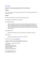
1 Nodes 10 Nodes 25 Nodes 50 Nodes 100 Nodes
0
250
500
750
1000
1250
1500
seconds


← 17.6
← 75.5
← 76.7
← 67.7
← 75.5
Vertica Hadoop
Figure 1: Load Times – Grep Task Data Set
(535MB/node)
25 Nodes 50 Nodes 100 Nodes

0
5000
10000
15000
20000
25000
30000
seconds


Vertica Hadoop
Figure 2: Load Times – Grep Task Data Set
(1TB/cluster)
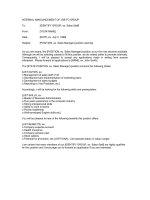
1 Nodes 10 Nodes 25 Nodes 50 Nodes 100 Nodes
0
10000
20000
30000
40000
50000
seconds


← 2262.2
← 4369.8
← 4445.3
← 4486.2
← 4520.8
Vertica Hadoop
Figure 3: Load Times – UserVisits Data Set

(20GB/node)
Since Hadoop needs a total of 3TB of disk space in order to store
three replicas of each block in HDFS, we were limited to running
this benchmark only on 25, 50, and 100 nodes (at fewer than 25
nodes, there is not enough available disk space to store 3TB).
4.2.1 Data Loading
We now describe the procedures used to load the data from the
nodes’ local files into each system’s internal storage representation.
Hadoop: There are two ways to load data into Hadoop’s distributed
file system: (1) use Hadoop’s command-line file utility to upload
files stored on the local filesystem into HDFS or (2) create a custom
data loader program that writes data using Hadoop’s internal I/O
API. We did not need to alter the input data for our MR programs,
therefore we loaded the files on each node in parallel directly into
HDFS as plain text using the command-line utility. Storing the data
in this manner enables MR programs to access data using Hadoop’s
TextInputFormat data format, where the keys are line num-
bers in each file and their corresponding values are the contents of
each line. We found that this approach yielded the best performance
in both the loading process and task execution, as opposed to using
Hadoop’s serialized data formats or compression features.
DBMS-X: The loading process in DBMS-X occurs in two phases.
First, we execute the LOAD SQL command in parallel on each node
in the cluster to read data from the local filesystem and insert its
contents into a particular table in the database. We specify in this
command that the local data is delimited by a special character, thus
we did not need to write a custom program to transform the data
before loading it. But because our data generator simply creates
random keys for each record on each node, the system must redis-
tribute the tuples to other nodes in the cluster as it reads each record

from the input files based on the target table’s partitioning attribute.
It would be possible to generate a “hash-aware” version of the data
generator that would allow DBMS-X to just load the input files on
each node without this redistribution process, but we do not believe
that this would improve load times very much.
Once the initial loading phase is complete, we then execute an
administrative command to reorganize the data on each node. This
process executes in parallel on each node to compress data, build
each table’s indexes, and perform other housekeeping.
Vertica: Vertica also provides a COPY SQL command that is is-
sued from a single host and then coordinates the loading process on
multiple nodes in parallel in the cluster. The user gives the COPY
command as input a list of nodes to execute the loading operation
for. This process is similar to DBMS-X: on each node the Vertica
loader splits the input data files on a delimiter, creates a new tuple
for each line in an input file, and redistributes that tuple to a dif-
ferent node based on the hash of its primary key. Once the data is
loaded, the columns are automatically sorted and compressed ac-
cording to the physical design of the database.
Results & Discussion: The results for loading both the 535MB/node
and 1TB/cluster data sets are shown in Figures 1 and 2, respectively.
For DBMS-X, we separate the times of the two loading phases,
which are shown as a stacked bar in the graphs: the bottom seg-
ment represents the execution time of the parallel LOAD commands
and the top segment is the reorganization process.
The most striking feature of the results for the load times in
535MB/node data set shown in Figure 1 is the difference in perfor-
mance of DBMS-X compared to Hadoop and Vertica. Despite issu-
ing the initial LOAD command in the first phase on each node in par-
allel, the data was actually loaded on each node sequentially. Thus,

as the total of amount of data is increased, the load times also in-
creased proportionately. This also explains why, for the 1TB/cluster
data set, the load times for DBMS-X do not decrease as less data
is stored per node. However, the compression and housekeeping on
DBMS-X can be done in parallel across nodes, and thus the execu-
tion time of the second phase of the loading process is cut in half
when twice as many nodes are used to store the 1TB of data.
Without using either block- or record-level compression, Hadoop
clearly outperforms both DBMS-X and Vertica since each node is
simply copying each data file from the local disk into the local
HDFS instance and then distributing two replicas to other nodes
in the cluster. If we load the data into Hadoop using only a sin-
gle replica per block, then the load times are reduced by a factor
of three. But as we will discuss in Section 5, the lack of multiple
replicas often increases the execution times of jobs.
4.2.2 Task Execution
SQL Commands: A pattern search for a particular field is sim-
ply the following query in SQL. Neither SQL system contained an
index on the field attribute, so this query requires a full table scan.
SELECT
*
FROM Data WHERE field LIKE ‘%XYZ%’;
MapReduce Program: The MR program consists of just a Map
function that is given a single record already split into the appro-
priate key/value pair and then performs a sub-string match on the
value. If the search pattern is found, the Map function simply out-
puts the input key/value pair to HDFS. Because no Reduce function
is defined, the output generated by each Map instance is the final
output of the program.
Results & Discussion: The performance results for the three sys-

tems for this task is shown in Figures 4 and 5. Surprisingly, the
relative differences between the systems are not consistent in the
1 Nodes 10 Nodes 25 Nodes 50 Nodes 100 Nodes
0
10
20
30
40
50
60
70
seconds


Vertica Hadoop
Figure 4: Grep Task Results – 535MB/node Data Set
25 Nodes 50 Nodes 100 Nodes
0
250
500
750
1000
1250
1500
seconds


Vertica Hadoop
Figure 5: Grep Task Results – 1TB/cluster Data Set
two figures. In Figure 4, the two parallel databases perform about

the same, more than a factor of two faster in Hadoop. But in Fig-
ure 5, both DBMS-X and Hadoop perform more than a factor of
two slower than Vertica. The reason is that the amount of data pro-
cessing varies substantially from the two experiments. For the re-
sults in Figure 4, very little data is being processed (535MB/node).
This causes Hadoop’s non-insignificant start-up costs to become the
limiting factor in its performance. As will be described in Section
5.1.2, for short-running queries (i.e., queries that take less than a
minute), Hadoop’s start-up costs can dominate the execution time.
In our observations, we found that takes 10–25 seconds before all
Map tasks have been started and are running at full speed across the
nodes in the cluster. Furthermore, as the total number of allocated
Map tasks increases, there is additional overhead required for the
central job tracker to coordinate node activities. Hence, this fixed
overhead increases slightly as more nodes are added to the cluster
and for longer data processing tasks, as shown in Figure 5, this fixed
cost is dwarfed by the time to complete the required processing.
The upper segments of each Hadoop bar in the graphs represent
the execution time of the additional MR job to combine the output
into a single file. Since we ran this as a separate MapReduce job,
these segments consume a larger percentage of overall time in Fig-
ure 4, as the fixed start-up overhead cost again dominates the work
needed to perform the rest of the task. Even though the Grep task is
selective, the results in Figure 5 show how this combine phase can
still take hundreds of seconds due to the need to open and combine
many small output files. Each Map instance produces its output in
a separate HDFS file, and thus even though each file is small there
are many Map tasks and therefore many files on each node.
For the 1TB/cluster data set experiments, Figure 5 shows that all
systems executed the task on twice as many nodes in nearly half the

amount of time, as one would expect since the total amount of data
was held constant across nodes for this experiment. Hadoop and
DBMS-X performs approximately the same, since Hadoop’s start-
up cost is amortized across the increased amount of data processing
for this experiment. However, the results clearly show that Vertica
outperforms both DBMS-X and Hadoop. We attribute this to Ver-
tica’s aggressive use of data compression (see Section 5.1.3), which
becomes more effective as more data is stored per node.
4.3 Analytical Tasks
To explore more complex uses of both types of systems, we de-
veloped four tasks related to HTML document processing. We first
generate a collection of random HTML documents, similar to that
which a web crawler might find. Each node is assigned a set of
600,000 unique HTML documents, each with a unique URL. In
each document, we randomly generate links to other pages set us-
ing a Zipfian distribution.
We also generated two additional data sets meant to model log
files of HTTP server traffic. These data sets consist of values de-
rived from the HTML documents as well as several randomly gen-
erated attributes. The schema of these three tables is as follows:
CREATE TABLE Documents (
url VARCHAR(100)
PRIMARY KEY,
contents TEXT );
CREATE TABLE Rankings (
pageURL VARCHAR(100)
PRIMARY KEY,
pageRank INT,
avgDuration INT );
CREATE TABLE UserVisits (

sourceIP VARCHAR(16),
destURL VARCHAR(100),
visitDate DATE,
adRevenue FLOAT,
userAgent VARCHAR(64),
countryCode VARCHAR(3),
languageCode VARCHAR(6),
searchWord VARCHAR(32),
duration INT );
Our data generator created unique files with 155 million UserVis-
its records (20GB/node) and 18 million Rankings records (1GB/node)
on each node. The visitDate, adRevenue, and sourceIP fields are
picked uniformly at random from specific ranges. All other fields
are picked uniformly from sampling real-world data sets. Each data
file is stored on each node as a column-delimited text file.
4.3.1 Data Loading
We now describe the procedures for loading the UserVisits and
Rankings data sets. For reasons to be discussed in Section 4.3.5,
only Hadoop needs to directly load the Documents files into its in-
ternal storage system. DBMS-X and Vertica both execute a UDF
that processes the Documents on each node at runtime and loads
the data into a temporary table. We account for the overhead of
this approach in the benchmark times, rather than in the load times.
Therefore, we do not provide results for loading this data set.
Hadoop: Unlike the Grep task’s data set, which was uploaded di-
rectly into HDFS unaltered, the UserVisits and Rankings data sets
needed to be modified so that the first and second columns are sep-
arated by a tab delimiter and all other fields in each line are sepa-
rated by a unique field delimiter. Because there are no schemas in
the MR model, in order to access the different attributes at run time,

the Map and Reduce functions in each task must manually split the
value by the delimiter character into an array of strings.
We wrote a custom data loader executed in parallel on each node
to read in each line of the data sets, prepare the data as needed,
and then write the tuple into a plain text file in HDFS. Loading
the data sets in this manner was roughly three times slower than
using the command-line utility, but did not require us to write cus-
1 Nodes 10 Nodes 25 Nodes 50 Nodes 100 Nodes
0
20
40
60
80
100
120
140
160
seconds


← 0.3
← 0.8
← 1.8
← 4.7
← 12.4
Vertica Hadoop
Figure 6: Selection Task Results
tom input handlers in Hadoop; the MR programs are able to use
Hadoop’s KeyValueTextInputFormat interface on the data
files to automatically split lines of text files into key/values pairs by

the tab delimiter. Again, we found that other data format options,
such as SequenceFileInputFormat or custom Writable
tuples, resulted in both slower load and execution times.
DBMS-X: We used the same loading procedures for DBMS-X as
discussed in Section 4.2. The Rankings table was hash partitioned
across the cluster on pageURL and the data on each node was sorted
by pageRank. Likewise, the UserVisits table was hash partitioned
on destinationURL and sorted by visitDate on each node.
Vertica: Similar to DBMS-X, Vertica used the same bulk load com-
mands discussed in Section 4.2 and sorted the UserVisits and Rank-
ings tables by the visitDate and pageRank columns, respectively.
Results & Discussion: Since the results of loading the UserVisits
and Ranking data sets are similar, we only provide the results for
loading the larger UserVisits data in Figure 3. Just as with loading
the Grep 535MB/node data set (Figure 1), the loading times for
each system increases in proportion to the number of nodes used.
4.3.2 Selection Task
The Selection task is a lightweight filter to find the pageURLs
in the Rankings table (1GB/node) with a pageRank above a user-
defined threshold. For our experiments, we set this threshold pa-
rameter to 10, which yields approximately 36,000 records per data
file on each node.
SQL Commands: The DBMSs execute the selection task using the
following simple SQL statement:
SELECT pageURL, pageRank
FROM Rankings WHERE pageRank > X;
MapReduce Program: The MR program uses only a single Map
function that splits the input value based on the field delimiter and
outputs the record’s pageURL and pageRank as a new key/value
pair if its pageRank is above the threshold. This task does not re-

quire a Reduce function, since each pageURL in the Rankings data
set is unique across all nodes.
Results & Discussion: As was discussed in the Grep task, the re-
sults from this experiment, shown in Figure 6, demonstrate again
that the parallel DBMSs outperform Hadoop by a rather significant
factor across all cluster scaling levels. Although the relative per-
formance of all systems degrade as both the number of nodes and
the total amount of data increase, Hadoop is most affected. For
example, there is almost a 50% difference in the execution time
between the 1 node and 10 node experiments. This is again due
to Hadoop’s increased start-up costs as more nodes are added to
the cluster, which takes up a proportionately larger fraction of total
query time for short-running queries.
Another important reason for why the parallel DBMSs are able
to outperform Hadoop is that both Vertica and DBMS-X use an in-
dex on the pageRank column and store the Rankings table already
sorted by pageRank. Thus, executing this query is trivial. It should
also be noted that although Vertica’s absolute times remain low, its
relative performance degrades as the number of nodes increases.
This is in spite of the fact that each node still executes the query in
the same amount of time (about 170ms). But because the nodes fin-
ish executing thequery so quickly, the system becomes flooded with
control messages from too many nodes, which then takes a longer
time for the system to process. Vertica uses a reliable message layer
for query dissemination and commit protocol processing [4], which
we believe has considerable overhead when more than a few dozen
nodes are involved in the query.
4.3.3 Aggregation Task
Our next task requires each system to calculate the total adRev-
enue generated for each sourceIP in the UserVisits table (20GB/node),

grouped by the sourceIP column. We also ran a variant of this query
where we grouped by the seven-character prefix of the sourceIP col-
umn to measure the effect of reducing the total number of groups
on query performance. We designed this task to measure the per-
formance of parallel analytics on a single read-only table, where
nodes need to exchange intermediate data with one another in order
compute the final value. Regardless of the number of nodes in the
cluster, this tasks always produces 2.5 million records (53 MB); the
variant query produces 2,000 records (24KB).
SQL Commands: The SQL commands to calculate the total adRev-
enue is straightforward:
SELECT sourceIP, SUM(adRevenue)
FROM UserVisits GROUP BY sourceIP;
The variant query is:
SELECT SUBSTR(sourceIP, 1, 7), SUM(adRevenue)
FROM UserVisits GROUP BY SUBSTR(sourceIP, 1, 7);
MapReduce Program: Unlike the previous tasks, the MR program
for this task consists of both a Map and Reduce function. The Map
function first splits the input value by the field delimiter, and then
outputs the sourceIP field (given as the input key) and the adRev-
enue field as a new key/value pair. For the variant query, only the
first seven characters (representing the first two octets, each stored
as three digits) of the sourceIP are used. These two Map functions
share the same Reduce function that simply adds together all of the
adRevenue values for each sourceIP and then outputs the prefix and
revenue total. We also used MR’s Combine feature to perform the
pre-aggregate before data is transmitted to the Reduce instances,
improving the first query’s execution time by a factor of two [8].
Results & Discussion: The results of the aggregation task experi-
ment in Figures 7 and 8 show once again that the two DBMSs out-

perform Hadoop. The DBMSs execute these queries by having each
node scan its local table, extract the sourceIP and adRevenue fields,
and perform a local group by. These local groups are then merged at
1 Nodes 10 Nodes 25 Nodes 50 Nodes 100 Nodes
0
200
400
600
800
1000
1200
1400
1600
1800
seconds


Vertica Hadoop
Figure 7: Aggregation Task Results (2.5 million Groups)
1 Nodes 10 Nodes 25 Nodes 50 Nodes 100 Nodes
0
200
400
600
800
1000
1200
1400
seconds

Vertica Hadoop
Figure 8: Aggregation Task Results (2,000 Groups)
the query coordinator, which outputs results to the user. The results
in Figure 7 illustrate that the two DBMSs perform about the same
for a large number of groups, as their runtime is dominated by the
cost to transmit the large number of local groups and merge them
at the coordinator. For the experiments using fewer nodes, Vertica
performs somewhat better, since it has to read less data (since it
can directly access the sourceIP and adRevenue columns), but it
becomes slightly slower as more nodes are used.
Based on the results in Figure 8, it is more advantageous to use
a column-store system when processing fewer groups for this task.
This is because the two columns accessed (sourceIP and adRev-
enue) consist of only 20 bytes out of the more than 200 bytes per
UserVisits tuple, and therefore there are relatively few groups that
need to be merged so communication costs are much lower than in
the non-variant plan. Vertica is thus able to outperform the other
two systems from not reading unused parts of the UserVisits tuples.
Note that the execution times for all systems are roughly consis-
tent for any number of nodes (modulo Vertica’s slight slow down as
the number of nodes increases). Since this benchmark task requires
the system to scan through the entire data set, the run time is always
bounded by the constant sequential scan performance and network
repartitioning costs for each node.
4.3.4 Join Task
The join task consists of two sub-tasks that perform a complex
calculation on two data sets. In the first part of the task, each sys-
tem must find the sourceIP that generated the most revenue within
a particular date range. Once these intermediate records are gener-

ated, the system must then calculate the average pageRank of all the
pages visited during this interval. We use the week of January 15-
22, 2000 in our experiments, which matches approximately 134,000
records in the UserVisits table.
The salient aspect of this task is that it must consume two data
different sets and join them together in order to find pairs of Rank-
ing and UserVisits records with matching values for pageURL and
destURL. This task stresses each system using fairly complex op-
erations over a large amount of data. The performance results are
also a good indication on how well the DBMS’s query optimizer
produces efficient join plans.
SQL Commands: In contrast to the complexity of the MR program
described below, the DBMSs need only two fairly simple queries to
complete the task. The first statement creates a temporary table and
uses it to store the output of the SELECT statement that performs
the join of UserVisits and Rankings and computes the aggregates.
Once this table is populated, it is then trivial to use a second query
to output the record with the largest totalRevenue field.
SELECT INTO Temp sourceIP,
AVG(pageRank) as avgPageRank,
SUM(adRevenue) as totalRevenue
FROM Rankings AS R, UserVisits AS UV
WHERE R.pageURL = UV.destURL
AND UV.visitDate BETWEEN Date(‘2000-01-15’)
AND Date(‘2000-01-22’)
GROUP BY UV.sourceIP;
SELECT sourceIP, totalRevenue, avgPageRank
FROM Temp
ORDER BY totalRevenue DESC LIMIT 1;
MapReduce Program: Because the MR model does not have an

inherent ability to join two or more disparate data sets, the MR pro-
gram that implements the join task must be broken out into three
separate phases. Each of these phases is implemented together as a
single MR program in Hadoop, but do not begin executing until the
previous phase is complete.
Phase 1
– The first phase filters UserVisits records that are outside
the desired data range and then joins the qualifying records with
records from the Rankings file. The MR program is initially given
all of the UserVisits and Rankings data files as input.
Map Function: For each key/value input pair, we determine its
record type by counting the number of fields produced when split-
ting the value on the delimiter. If it is a UserVisits record, we
apply the filter based on the date range predicate. These qualify-
ing records are emitted with composite keys of the form (destURL,
K
1
), where K
1
indicates that it is a UserVisits record. All Rankings
records are emitted with composite keys of the form (pageURL,
K
2
), where K
2
indicates that it is a Rankings record. These output
records are repartitioned using a user-supplied partitioning function
that only hashes on the URL portion of the composite key.
Reduce Function: The input to the Reduce function is a single
sorted run of records in URL order. For each URL, we divide its

values into two sets based on the tag component of the composite
key. The function then forms the cross product of the two sets to
complete the join and outputs a new key/value pair with the sour-
ceIP as the key and the tuple (pageURL, pageRank, adRevenue) as
the value.
Phase 2
– The next phase computes the total adRevenue and aver-
age pageRank based on the sourceIP of records generated in Phase
1. This phase uses a Reduce function in order to gather all of the
1 Nodes 10 Nodes 25 Nodes 50 Nodes 100 Nodes
0
200
400
600
800
1000
1200
1400
1600
1800
seconds


← 21.5
← 28.2
← 31.3
← 36.1
← 85.0
← 15.7
← 28.0

← 29.2
← 29.4
← 31.9
Vertica DBMS−X Hadoop
Figure 9: Join Task Results
1 Nodes 10 Nodes 25 Nodes 50 Nodes 100 Nodes
0
1000
2000
3000
4000
5000
6000
7000
8000
seconds


Vertica Hadoop
Figure 10: UDF Aggregation Task Results
records for a particular sourceIP on a single node. We use the iden-
tity Map function in the Hadoop API to supply records directly to
the split process [1, 8].
Reduce Function: For each sourceIP, the function adds up the
adRevenue and computes the average pageRank, retaining the one
with the maximum total ad revenue. Each Reduce instance outputs
a single record with sourceIP as the key and the value as a tuple of
the form (avgPageRank, totalRevenue).
Phase 3 – In the final phase, we again only need to define a sin-
gle Reduce function that uses the output from the previous phase to

produce the record with the largest total adRevenue. We only exe-
cute one instance of the Reduce function on a single node to scan
all the records from Phase 2 and find the target record.
Reduce Function: The function processes each key/value pair
and keeps track of the record with the largest totalRevenue field.
Because the Hadoop API does not easily expose the total number
records that a Reduce instance will process, there is no way for
the Reduce function to know that it is processing the last record.
Therefore, we override the closing callback method in our Reduce
implementation so that the MR program outputs the largest record
right before it exits.
Results & Discussion: The performance results for this task is dis-
played in Figure 9. We had to slightly change the SQL used in 100
node experiments for Vertica due to an optimizer bug in the system,
which is why there is an increase in the execution time for Vertica
going from 50 to 100 nodes. But even with this increase, it is clear
that this task results in the biggest performance difference between
Hadoop and the parallel database systems. The reason for this dis-
parity is two-fold.
First, despite the increased complexity of the query, the perfor-
mance of Hadoop is yet again limited by the speed with which the
large UserVisits table (20GB/node) can be read off disk. The MR
program has to perform a complete table scan, while the parallel
database systems were able to take advantage of clustered indexes
on UserVisits.visitDate to significantly reduce the amount of data
that needed to be read. When breaking down the costs of the dif-
ferent parts of the Hadoop query, we found that regardless of the
number of nodes in the cluster, phase 2 and phase 3 took on aver-
age 24.3 seconds and 12.7 seconds, respectively. In contrast, phase
1, which contains the Map task that reads in the UserVisits and

Rankings tables, takes an average of 1434.7 seconds to complete.
Interestingly, it takes approximately 600 seconds of raw I/O to read
the UserVisits and Rankings tables off of disk and then another 300
seconds to split, parse, and deserialize the various attributes. Thus,
the CPU overhead needed to parse these tables on the fly is the lim-
iting factor for Hadoop.
Second, the parallel DBMSs are able to take advantage of the fact
that both the UserVisits and the Rankings tables are partitioned by
the join key. This means that both systems are able to do the join
locally on each node, without any network overhead of repartition-
ing before the join. Thus, they simply have to do a local hash join
between the Rankings table and a selective part of the UserVisits
table on each node, with a trivial ORDER BY clause across nodes.
4.3.5 UDF Aggregation Task
The final task is to compute the inlink count for each document
in the dataset, a task that is often used as a component of PageR-
ank calculations. Specifically, for this task, the systems must read
each document file and search for all the URLs that appear in the
contents. The systems must then, for each unique URL, count the
number of unique pages that reference that particular URL across
the entire set of files. It is this type of task that the MR is believed
to be commonly used for.
We make two adjustments for this task in order to make pro-
cessing easier in Hadoop. First, we allow the aggregate to include
self-references, as it is non-trivial for a Map function to discover
the name of the input file it is processing. Second, on each node
we concatenate the HTML documents into larger files when storing
them in HDFS. We found this improved Hadoop’s performance by
a factor of two and helped avoid memory issues with the central
HDFS master when a large number of files are stored in the system.

SQL Commands: To perform this task in a parallel DBMS re-
quires a user-defined function F that parses the contents of each
record in the Documents table and emits URLs into the database.
This function can be written in a general-purpose language and is
effectively identical to the Map program discussed below. With this
function F, we populate a temporary table with a list of URLs and
then can execute a simple query to calculate the inlink count:
SELECT INTO Temp F(contents) FROM Documents;
SELECT url, SUM(value) FROM Temp GROUP BY url;
Despite the simplicity of this proposed UDF, we found that in
practice it was difficult to implement in the DBMSs.
For DBMS-X, we translated the MR program used in Hadoop
into an equivalent C program that uses the POSIX regular expres-
sion library to search for links in the document. For each URL
found in the document contents, the UDF returns a new tuple (URL,
1) to the database engine. We originally intended to store each
HTML document as a character BLOB in DBMS-X and then exe-
cute the UDF on each document completely inside of the database,
but were unable to do so due to a known bug in our version of the
system. Instead, we modified the UDF to open each HTML docu-
ment on the local disk and process its contents as if it was stored
in the database. Although this is similar to the approach that we
had to take with Vertica (see below), the DBMS-X UDF did not
run as an external process to the database and did not require any
bulk-loading tools to import the extracted URLs.
Vertica does not currently support UDFs, therefore we had to
implement this benchmark task in two phases. In the first phase,
we used a modified version of DBMS-X’s UDF to extract URLs
from the files, but then write the output to files on each node’s lo-
cal filesystem. Unlike DBMS-X, this program executes as a sepa-

rate process outside of the database system. Each node then loads
the contents of these files into a table using Vertica’s bulk-loading
tools. Once this is completed, we then execute the query as de-
scribed above to compute the inlink count for each URL.
MapReduce Program: To fit into the MR model where all data
must be defined in terms of key/value pairs, each HTML document
is split by its lines and given to the Map function with the line con-
tents as the value and the line number in which it appeared in the
file as its key. The Map function then uses a regular expression to
find all of the URLs in each line. For every URL found, the function
outputs the URL and the integer 1 as a new key/value pair. Given
these records, the Reduce function then simply counts the number
of values for a given key and outputs the URL and the calculated
inlink count as the program’s final output.
Results & Discussion: The results in Figure 10 show that both
DBMS-X and Hadoop (not including the extra Reduce process to
combine the data) have approximately constant performance for
this task, since each node has the same amount of Document data
to process and this amount of data remains constant (7GB) as more
nodes are added in the experiments. As we expected, the additional
operation for Hadoop to combine data into a single file in HDFS
gets progressively slower since the amount of output data that the
single node must process gets larger as new nodes are added. The
results for both DBMS-X and Vertica are shown in Figure 10 as
stacked bars, where the bottom segment represents the time it took
to execute the UDF/parser and load the data into the table and the
top segment is the time to execute the actual query. DBMS-X per-
forms worse than Hadoop due to the added overhead of row-by-row
interaction between the UDF and the input file stored outside of the
database. Vertica’s poor performance is the result of having to parse

data outside of the DBMS and materialize the intermediate results
on the local disk before it can load it into the system.
5. DISCUSSION
We now discuss broader issues about the benchmark results and
comment on particular aspects of each system that the raw numbers
may not convey. In the benchmark above, both DBMS-X and Ver-
tica execute most of the tasks much faster than Hadoop at all scaling
levels. The next subsections describe, in greater detail than the pre-
vious section, the reasons for this dramatic performance difference.
5.1 System-level Aspects
In this section, we describe how architectural decisions made at
the system-level affect the relative performance of the two classes of
data analysis systems. Since installation and configuration param-
eters can have a significant difference in the ultimate performance
of the system, we begin with a discussion of the relative ease with
which these parameters are set. Afterwards, we discuss some lower
level implementation details. While some of these details affect
performance in fundamental ways (e.g., the fact that MR does not
transform data on loading precludes various I/O optimizations and
necessitates runtime parsing which increases CPU costs), others are
more implementation specific (e.g., the high start-up cost of MR).
5.1.1 System Installation, Configuration, and Tuning
We were able to get Hadoop installed and running jobs with little
effort. Installing the system only requires setting up data directories
on each node and deploying the system library and configuration
files. Configuring the system for optimal performance was done
through trial and error. We found that certain parameters, such as
the size of the sort buffers or the number of replicas, had no affect
on execution performance, whereas other parameters, such as using
larger block sizes, improved performance significantly.

The DBMS-X installation process was relatively straightforward.
A GUI leads the user through the initial steps on one of the cluster
nodes, and then prepares afile that can be fed to an installer utility in
parallel on the other nodes to complete the installation. Despite this
simple process, we found that DBMS-X was complicated to config-
ure in order to start running queries. Initially, we were frustrated by
the failure of anything but the most basic of operations. We eventu-
ally discovered each node’s kernel was configured to limit the total
amount of allocated virtual address space. When this limit was hit,
new processes could not be created and DBMS-X operations would
fail. We mention this even though it was our own administrative er-
ror, as we were surprised that DBMS-X’s extensive system probing
and self-adjusting configuration was not able to detect this limita-
tion. This was disappointing after our earlier Hadoop successes.
Even after these earlier issues were resolved and we had DBMS-
X running, we were routinely stymied by other memory limitations.
We found that certain default parameters, such as the sizes of the
buffer pool and sort heaps, were too conservative for modern sys-
tems. Furthermore, DBMS-X proved to be ineffective at adjusting
memory allocations for changing conditions. For example, the sys-
tem automatically expanded our buffer pool from the default 4MB
to only 5MB (we later forced it to 512 MB). It also warned us that
performance could be degraded when we increased our sort heap
size to 128 MB (in fact, performance improved by a factor of 12).
Manually changing some options resulted in the system automat-
ically altering others. On occasion, this combination of manual
and automatic changes resulted in a configuration for DBMS-X that
caused it to refuse to boot the next time the system started. As most
configuration settings required DBMS-X to be running in order to
adjust them, it was unfortunately easy to lock ourselves out with no

failsafe mode to restore to a previous state.
Vertica was relatively easy to install as an RPM that we deployed
on each node. An additional configuration script bundled with the
RPM is used to build catalog meta-data and modify certain kernel
parameters. Database tuning is minimal and is done through hints
to the resource manager; we found that the default settings worked
well for us. The downside of this simplified tuning approach, how-
ever, is that there is no explicit mechanism to determine what re-
sources were granted to a query nor is there a way to manually
adjust per query resource allocation.
The take-away from our efforts is that we found parallel DBMSs
to be much more challenging than Hadoop to install and configure
properly. There is, however, a significant variation with respect to
ease of installation and configuration across the different parallel
database products. One small advantage for the database systems is
that the tuning that is needed is mostly done prior to query execu-
tion, and that certain tuning parameters (e.g., sort buffer sizes) are
suitable for all tasks. In contrast, for Hadoop we not only had to
tune the system (e.g., block sizes), but we also occasionally needed
to tune each individual task to work well with the system (e.g.,
changing code). Finally, the parallel database products came with
tools to aid in the tuning process whereas with Hadoop we were
forced to resort to trial and error tuning; clearly a more mature MR
implementation could include such tuning tools as well.
5.1.2 Task Start-up
We found that our MR programs took some time before all nodes
were running at full capacity. On a cluster of 100 nodes, it takes 10
seconds from the moment that a job is submitted to the JobTracker
before the first Map task begins to execute and 25 seconds until all
the nodes in the cluster are executing the job. This coincides with

the results in [8], where the data processing rate does not reach its
peak for nearly 60 seconds on a cluster of 1800 nodes. The “cold
start” nature is symptomatic to Hadoop’s (and apparently Google’s)
implementation and not inherent to the actual MR model itself. For
example, we also found that prior versions of Hadoop would create
a new JVM process for each Map and Reduce instance on a node,
which we found increased the overhead of running jobs on large
data sets; enabling the JVM reuse feature in the latest version of
Hadoop improved our results for MR by 10–15%.
In contrast, parallel DBMSs are started at OS boot time, and thus
are considered to always be “warm”, waiting for a query to execute.
Moreover, all modern DBMSs are designed to execute using multi-
ple threads and processes, which allows the currently running code
to accept additional tasks and further optimize its execution sched-
ule. Minimizing start-up time was one of the early optimizations of
DBMSs, and is certainly something that MR systems should be able
to incorporate without a large rewrite of the underlying architecture.
5.1.3 Compression
Almost every parallel DBMS (including DBMS-X and Vertica)
allows for optional compression of stored data. It is not uncom-
mon for compression to result in a factor of 6–10 space savings.
Vertica’s internal data representation is highly optimized for data
compression and has an execution engine that operates directly on
compressed data (i.e., it avoids decompressing the data during pro-
cessing whenever possible). In general, since analysis tasks on large
data sets are often I/O bound, trading CPU cycles (needed to de-
compress input data) for I/O bandwidth (compressed data means
that there is less data to read) is a good strategy and translates to
faster execution. In situations where the executor can operate di-
rectly on compressed data, there is often no trade-off at all and

compression is an obvious win.
Hadoop and its underlying distributed filesystem support both
block-level and record-level compression on input data. We found,
however, that neither technique improved Hadoop’s performance
and in some cases actually slowed execution. It also required more
effort on our part to either change code or prepare the input data.
It should also be noted that compression was also not used in the
original MR benchmark [8].
In order to use block-level compression in Hadoop, we first had
to split the data files into multiple, smaller files on each node’s local
file system and then compress each file using the gzip tool. Com-
pressing the data in this manner reduced each data set by 20–25%
from its original size. These compressed files are then copied into
HDFS just as if they were plain text files. Hadoop automatically
detects when files are compressed and will decompress them on the
fly when they are fed into Map instances, thus we did not need to
change our MR programs to use the compressed data. Despite the
longer load times (if one includes the splitting and compressing),
Hadoop using block-level compression slowed most the tasks by a
few seconds while CPU-bound tasks executed 50% slower.
We also tried executing the benchmarks using record-level com-
pression. This required us to (1) write to a custom tuple object us-
ing Hadoop’s API, (2) modify our data loader program to transform
records to compressed and serialized custom tuples, and (3) refac-
tor each benchmark. We initially believed that this would improve
CPU-bound tasks, because the Map and Reduce tasks no longer
needed to split the fields by the delimiter. We found, however, that
this approach actually performed worse than block-level compres-
sion while only compressing the data by 10%.
5.1.4 Loading and Data Layout

Parallel DBMSs have the opportunity to reorganize the input data
file at load time. This allows for certain optimizations, such as stor-
ing each attribute of a table separately (as done in column-stores
such as Vertica). For read-only queries that only touch a subset of
the attributes of a table, this optimization can improve performance
by allowing the attributes that are not accessed by a particular query
to be left on disk and never read. Similar to the compression opti-
mization described above, this saves critical I/O bandwidth. MR
systems by default do not transform the data when it is loaded into
their distributed file system, and thus are unable to change the lay-
out of input data, which precludes this class of optimization oppor-
tunities. Furthermore, Hadoop was always much more CPU inten-
sive than the parallel DBMS in running equivalent tasks because
it must parse and deserialize the records in the input data at run
time, whereas parallel databases do the parsing at load time and can
quickly extract attributes from tuples at essentially zero cost.
But MR’s simplified loading process did make it much easier
and faster to load than with the DBMSs. Our results in Sections
4.2.1 and 4.3.1 show that Hadoop achieved load throughputs of up
to three times faster than Vertica and almost 20 times faster than
DBMS-X. This suggests that for data that is only going to be loaded
once for certain types on analysis tasks, that it may not be worth it
to pay the cost of the indexing and reorganization cost in a DBMS .
This also strongly suggests that a DBMS would benefit from a “in-
situ” operation mode that would allow a user to directly access and
query files stored in a local file system.
5.1.5 Execution Strategies
As noted earlier, the query planner in parallel DBMSs are care-
ful to transfer data between nodes only if it is absolutely necessary.
This allows the systems to optimize the join algorithm depending

on the characteristics of the data and perform push-oriented mes-
saging without writing intermediate data sets. Over time, MR ad-
vocates should study the techniques used in parallel DBMSs and
incorporate the concepts that are germane to their model. In doing
so, we believe that again the performance of MR frameworks will
improve dramatically.
Furthermore, parallel DBMSs construct a complete query plan
that is sent to all processing nodes at the start of the query. Because
data is “pushed” between sites when only necessary, there are no
control messages during processing. In contrast, MR systems use a
large number of control messages to synchronize processing, result-
ing in poorer performance due to increased overhead; Vertica also
experienced this problem but on a much smaller scale (Section 4.2).
5.1.6 Failure Model
As discussed previously, while not providing support for transac-
tions, MR is able to recover from faults in the middle of query ex-
ecution in a way that most parallel database systems cannot. Since
parallel DBMSs will be deployed on larger clusters over time, the
probability of mid-query hardware failures will increase. Thus, for
long running queries, it may be important to implement such a fault
tolerance model. While improving the fault-tolerance of DBMSs is
clearly a good idea, we are wary of devoting huge computational
clusters and “brute force” approaches to computation when sophis-
ticated software would could do the same processing with far less
hardware and consume far less energy, or in less time, thereby ob-
viating the need for a sophisticated fault tolerance model. A multi-
thousand-node cluster of the sort Google, Microsoft, and Yahoo!
run uses huge amounts of energy, and as our results show, for many
data processing tasks a parallel DBMS can often achieve the same
performance using far fewer nodes. As such, the desirable ap-

proach is to use high-performance algorithms with modest paral-
lelism rather than brute force approaches on much larger clusters.
5.2 User-level Aspects
A data processing system’s performance is irrelevant to a user
or an organization if the system is not usable. In this section, we
discuss aspects of each system that we encountered from a user-
level perspective while conducting the benchmark study that may
promote or inhibit application development and adoption.
5.2.1 Ease of Use
Once the system is on-line and the data has been loaded, the pro-
grammer then begins to write the query or the code needed to per-
form their task. Like other kinds of programming, this is often an
iterative process: the programmer writes a little bit of code, tests it,
and then writes some more. The programmer can easily determine
whether his/her code is syntactically correct in both types of sys-
tems: the MR framework can check whether the user’s code com-
piles and the SQL engines can determine whether the queries parse
correctly. Both systems also provide runtime support to assist users
in debugging their programs.
It is also worth considering the way in which the programmer
writes the query. MR programs in Hadoop are primarily written in
Java (though other language bindings exist). Most programmers are
more familiar with object-oriented, imperative programming than
with other language technologies, such as SQL. That said, SQL
is taught in many undergraduate programs and is fairly portable –
we were able to share the SQL commands between DBMS-X and
Vertica with only minor modifications.
In general, we found that getting an MR program up and running
with Hadoop took less effort than with the other systems. We did
not need to construct a schema or register user-defined functions in

order to begin processing the data. However, after obtaining our
initial results, we expanded the number of benchmark tasks, caus-
ing us to add new columns to our data set. In order to process
this new data, we had to modify our existing MR code and retest
each MR program to ensure that it worked with the new assump-
tions about the data’s schema. Furthermore, some API methods in
Hadoop were deprecated after we upgraded to newer versions of
the system, which again required us to rewrite portions of our pro-
grams. In contrast, once we had built our initial SQL-based appli-
cations, we did not have to modify the code despite several changes
to our benchmark schema.
We argue that although it may be easier to for developers to get
started with MR, maintenance of MR programs is likely to lead to
significant pain for applications developers over time. As we also
argued in Section 3.1, reusing MR code between two deployments
or on two different data sets is difficult, as there is no explicit rep-
resentation of the schema for data used in the MR model.
5.2.2 Additional Tools
Hadoop comes with a rudimentary web interface that allows the
user to browse the contents of the distributed filesystem and monitor
the execution of jobs. Any additional tools would most likely at this
time have to be developed in house.
SQL databases, on the other hand, have tons of existing tools and
applications for reporting and data analysis. Entire software indus-
tries have developed around providing DBMS users with third-party
extensions. The types of software that many of these tools include
(1) data visualization, (2) business intelligence, (3) data mining, (4)
data replication, and (5) automatic database design. Because MR
technologies are still nascent, the market for such software for MR
is limited; however, as the user base grows, many of the existing

SQL-based tools will likely support MR systems.
6. CONCLUSION
There are a number of interesting conclusions that can be drawn
from the results presented in this paper. First, at the scale of the ex-
periments we conducted, both parallel database systems displayed a
significant performance advantage over Hadoop MR in executing a
variety of data intensive analysis benchmarks. Averaged across all
five tasks at 100 nodes, DBMS-X was 3.2 times faster than MR and
Vertica was 2.3 times faster than DBMS-X. While we cannot verify
this claim, we believe that the systems would have the same relative
performance on 1,000 nodes (the largest Teradata configuration is
less than 100 nodes managing over four petabytes of data). The dual
of these numbers is that a parallel database system that provides the
same response time with far fewer processors will certainly uses far
less energy; the MapReduce model on multi-thousand node clusters
is a brute force solution that wastes vast amounts of energy. While it
is rumored that the Google version of MR is faster than the Hadoop
version, we did not have access to this code and hence could not test
it. We are doubtful again, however, that there would be a substantial
difference in the performance of the two versions as MR is always
forced to start a query with a scan of the entire input file.
This performance advantage that the two database systems share
is the result of a number of technologies developed over the past
25 years, including (1) B-tree indices to speed the execution of
selection operations, (2) novel storage mechanisms (e.g., column-
orientation), (3) aggressive compression techniques with ability to
operate directly on compressed data, and (4) sophisticated parallel
algorithms for querying large amounts of relational data. In the case
of a column-store database like Vertica, only those columns that are
needed to execute a query are actually read from disk. Furthermore,

the column-wise storage of data results in better compression fac-
tors (approximately a factor of 2.0 for Vertica, versus a factor of 1.8
for DBMS-X and 1.25 for Hadoop); this also further reduces the
amount of disk I/O that is performed to execute a query.
Although we were not surprised by the relative performance ad-
vantages provided by the two parallel database systems, we were
impressed by how easy Hadoop was to set up and use in comparison
to the databases. The Vertica installation process was also straight-
forward but temperamental to certain system parameters. DBMS-
X, on the other hand, was difficult to configure properly and re-
quired repeated assistance from the vendor to obtain a configuration
that performed well. For a mature product such as DBMS-X, the
entire experience was indeed disappointing. Given the upfront cost
advantage that Hadoop has, we now understand why it has quickly
attracted such a large user community.
Extensibility was another area where we found the database sys-
tems we tested lacking. Extending a DBMS with user-defined types
and functions is an idea that is now 25 years old [16]. Neither of
the parallel systems we tested did a good job on the UDF aggre-
gation tasks, forcing us to find workarounds when we encountered
limitations (e.g., Vertica) and bugs (e.g., DBMS-X).
While all DB systems are tolerant of a wide variety of software
failures, there is no question that MR does a superior job of mini-
mizing the amount of work that is lost when a hardware failure oc-
curs. This capability, however, comes with a potentially large per-
formance penalty, due to the cost of materializing the intermediate
files between the map and reduce phases. Left unanswered is how
significant this performance penalty is. Unfortunately, to investi-
gate this question properly requires implementing both the materi-
alization and no-materialization strategies in a common framework,

which is an effort beyond the scope of this paper. Despite a clear
advantage in this domain, it is not completely clear how significant
a factor Hadoop’s ability to tolerate failures during execution really
is in practice. In addition, if a MR system needs 1,000 nodes to
match the performance of a 100 node parallel database system, it is
ten times more likely that a node will fail while a query is execut-
ing. That said, better tolerance to failures is a capability that any
database user would appreciate.
Many people find SQL difficult to use initially. This is partially
due to having to think differently when solving a problem and that
SQL has evolved into a complex language that is quite different than
the original design by Don Chamberlin in the 1970s. Though most
languages become more complex over time, SQL is particularly bad
as many of its features were designed by competing database com-
panies who each sought to include their own proprietary extensions.
Despite its faults, SQL is still a powerful tool. Consider the
following query to generate a list of Employees ordered by their
salaries and the corresponding rank of each salary (i.e., the highest
paid employee gets a rank of one):
SELECT Emp.name, Emp.salary,
RANK() OVER (ORDER BY Emp.salary)
FROM Employees AS Emp
Computing this in parallel requires producing a total order of
all employees followed by a second phase in which each node ad-
justs the rank values of its records with the counts of the number
of records on each node to its “left” (i.e., those nodes with salary
values that are strictly smaller). Although a MR program could per-
form this sort in parallel, it is not easy to fit this query into the MR
paradigm of group by aggregation. RANK is just one of the many
powerful analytic functions provided by modern parallel database

systems. For example, both Teradata and Oracle support a rich set
of functions, such as functions over windows of ordered records.
Two architectural differences are likely to remain in the long run.
MR makes a commitment to a “schema later” or even “schema
never” paradigm. But this lack of a schema has a number of im-
portant consequences. Foremost, it means that parsing records at
run time is inevitable, in contrast to DBMSs, which perform pars-
ing at load time. This difference makes compression less valuable
in MR and causes a portion of the performance difference between
the two classes of systems. Without a schema, each user must write
a custom parser, complicating sharing data among multiple applica-
tions. Second, a schema is needed for maintaining information that
is critical for optimizing declarative queries, including what indices
exist, how tables are partitioned, table cardinalities, and histograms
that capture the distribution of values within a column.
In our opinion there is a lot to learn from both kinds of systems.
Most importantly is that higher level interfaces, such as Pig [15],
Hive [2], are being put on top of the MR foundation, and a number
of tools similar in spirit but more expressive than MR are being de-
veloped, such as Dryad [13] and Scope [5]. This will make complex
tasks easier to code in MR-style systems and remove one of the big
advantages of SQL engines, namely that they take much less code
on the tasks in our benchmark. For parallel databases, we believe
that both commercial and open-source systems will dramatically
improve the parallelization of user-defined functions. Hence, the
APIs of the two classes of systems are clearly moving toward each
other. Early evidence of this is seen in the solutions for integrating
SQL with MR offered by Greenplum and Asterdata.
7. ACKNOWLEDGMENTS
The authors would like to thank Lakshmikant Shrinivas in help-

ing to get DBMS-X running, as well as Chris Olston and the re-
viewers for their insightful comments and feedback. This work was
supported in part by NSF Grant CluE - 0844013/0844480.
8. REFERENCES
[1] Hadoop. />[2] Hive. />[3] Vertica. />[4] Y. Amir and J. Stanton. The Spread Wide Area Group
Communication System. Technical report, 1998.
[5] R. Chaiken, B. Jenkins, P A. Larson, B. Ramsey, D. Shakib,
S. Weaver, and J. Zhou. Scope: easy and efficient parallel
processing of massive data sets. Proc. VLDB Endow.,
1(2):1265–1276, 2008.
[6] Cisco Systems. Cisco Catalyst 3750-E Series Switches Data
Sheet, June 2008.
[7] J. Cohen, B. Dolan, M. Dunlap, J. M. Hellerstein, and
C. Welton. MAD Skills: New Analysis Practices for Big
Data. Under Submission, March 2009.
[8] J. Dean and S. Ghemawat. MapReduce: Simplified Data
Processing on Large Clusters. In OSDI ’04, pages 10–10,
2004.
[9] D. J. DeWitt and R. H. Gerber. Multiprocessor Hash-based
Join Algorithms. In VLDB ’85, pages 151–164, 1985.
[10] D. J. DeWitt, R. H. Gerber, G. Graefe, M. L. Heytens, K. B.
Kumar, and M. Muralikrishna. GAMMA - A High
Performance Dataflow Database Machine. In VLDB ’86,
pages 228–237, 1986.
[11] S. Fushimi, M. Kitsuregawa, and H. Tanaka. An Overview of
The System Software of A Parallel Relational Database
Machine. In VLDB ’86, pages 209–219, 1986.
[12] S. Ghemawat, H. Gobioff, and S T. Leung. The Google File
System. SIGOPS Oper. Syst. Rev., 37(5):29–43, 2003.
[13] M. Isard, M. Budiu, Y. Yu, A. Birrell, and D. Fetterly. Dryad:

Distributed Data-parallel Programs from Sequential Building
Blocks. In EuroSys ’07, pages 59–72, 2007.
[14] E. Meijer, B. Beckman, and G. Bierman. LINQ: reconciling
object, relations and XML in the .NET framework. In
SIGMOD ’06, pages 706–706, 2006.
[15] C. Olston, B. Reed, U. Srivastava, R. Kumar, and
A. Tomkins. Pig Latin: A Not-So-Foreign Language for Data
Processing. In SIGMOD ’08, pages 1099–1110, 2008.
[16] J. Ong, D. Fogg, and M. Stonebraker. Implementation of data
abstraction in the relational database system ingres. SIGMOD
Rec., 14(1):1–14, 1983.
[17] D. A. Patterson. Technical Perspective: The Data Center is
the Computer. Commun. ACM, 51(1):105–105, 2008.
[18] R. Rustin, editor. ACM-SIGMOD Workshop on Data
Description, Access and Control, May 1974.
[19] M. Stonebraker. The Case for Shared Nothing. Database
Engineering, 9:4–9, 1986.
[20] M. Stonebraker and J. Hellerstein. What Goes Around
Comes Around. In Readings in Database Systems, pages
2–41. The MIT Press, 4th edition, 2005.
[21] D. Thomas, D. Hansson, L. Breedt, M. Clark, J. D. Davidson,
J. Gehtland, and A. Schwarz. Agile Web Development with
Rails. Pragmatic Bookshelf, 2006.