Tài liệu Aesthetic Visual Quality Assessment of Paintings doc

> REPLACE THIS LINE WITH YOUR PAPER IDENTIFICATION NUMBER (DOUBLE-CLICK HERE TO EDIT) <

1

Abstract— This paper aims to evaluate the aesthetic visual
quality of a special type of visual media: digital images of paintings.
Assessing the aesthetic visual quality of paintings can be
considered a highly subjective task. However, to some extent,
certain paintings are believed, by consensus, to have higher
aesthetic quality than others. In this paper, we treat this challenge
as a machine learning problem, in order to evaluate the aesthetic
quality of paintings based on their visual content. We design a
group of methods to extract features to represent both the global
characteristics and local characteristics of a painting. Inspiration
for these features comes from our prior knowledge in art and a
questionnaire survey we conducted to study factors that affect
human’s judgments. We collect painting images and ask human
subjects to score them. These paintings are then used for both
training and testing in our experiments. Experiment results show
that the proposed work can classify high-quality and low-quality
paintings with performance comparable to humans. This work
provides a machine learning scheme for the research of exploring
the relationship between aesthetic perceptions of human and the
computational visual features extracted from paintings.

Index Terms— Visual Quality Assessment, Aesthetics, Feature
Extraction, Classification

I. I
NTRODUCTION
he booming development of digital media has changed the

modern life a lot. It not only introduces more approaches
for human to see and feel about the world, but also changes
the ways that computer “sees” and “feels”. It raises a group of
interesting topics about allowing a computer to see and feel as
human beings. For example, in the field of compression, lots of
metrics have been proposed to allow a computer to evaluate the
visual quality of the compressed images/videos and come to
conclusions in accordance with human’s subjective evaluations.
We can see that these metrics are all aiming to measure the
visual quality degradation caused by compression artifacts,
which is mainly dependent on the compression techniques.
However, this is only one aspect of visual quality. Visual quality
as a whole can be more complex, which not only includes the
visual effect that is due to techniques used in digitalization, but
also include other aspects that are relevant with the content of
the visual object itself. In this paper, we focus on the visual
quality on the aspect of aesthetics. As known to us, judging the
aesthetic quality is always an important part of human’s opinion

Congcong Li is with Electrical and Computer Engineering Department,
Carnegie Mellon University, Pittsburgh, PA 15213 USA (e-mail:

; Phone: 412-268-7115 ).
Tsuhan Chen is with the school of Electrical and Computer Engineering,
Cornell University, Ithaca, NY 14853 USA. (e-mail:
;
Phone: 607-255-5728).
towards what they see. The visual objects to be evaluated in this
paper are paintings, more exactly, digital images of paintings.
The motivation for evaluating the aesthetic visual quality on

paintings is not only to build a bridge between computer vision
and human perception, but also to build a bridge between
computer vision and art works.

A. Aesthetic Visual Quality Assessment of Paintings
1) Definition
Aesthetic visual quality assessment of painting is to evaluate
a painting in the sense of visual aesthetics. That is, we would
like to allow the computer to judge whether a painting is
beautiful or not in human’s eyes. Therefore, different from the
visual quality related to the degradation due to compression
artifacts, the aesthetic quality is mainly related to the visual
content itself – in this paper, the visual content of a painting.

2) Motivations
In the past, to evaluate the visual quality related to the content
can only be done on-site because digital media were not
available. However, with the trend of information digitalization,
digital images of paintings can be easily found on the internet.
This makes it possible for computers to do the evaluation. At the
same time, common people now have more opportunities to
appreciate art works casually without going to museums since
online art libraries or galleries are emerging. Inside these
systems, knowing the favorable degree of each painting will be
very helpful for painting image management, painting search
and painting recommendation. However, as we can imagine, it
is impossible to ask people to evaluate a gallery of thousands of
paintings. Instead, efficient evaluation by a computer will help
in solving these problems.
Another motivation for evaluating aesthetic quality on

paintings is to help popular-style artists and designers to know
about the potential opinions of viewers or users more easily.
Since art is no longer luxurious enjoyment for a charmed circle,
it has pervaded common people’s life and different areas.
What’s more, in recent years, favorable styles or patterns of
paintings are widely introduced into the appearance design of
architecture, product, and clothes etc. The spread of the
post-impressionist Piet Mondrian’s painting style into
architecture and furniture is one typical example. Therefore,
with automatic aesthetic quality analysis, designers and
popular-art artists will have one more guidelines to evaluate
their ideas in the designing course.
In addition to the above motivations towards applications,
another motivation for this research is to get a better
understanding of human vision in the aspect of aesthetics – to
find out whether there is any pattern that can represent human
Aesthetic Visual Quality Assessment of Paintings
Congcong Li, Student Member, IEEE, and Tsuhan Chen, Fellow, IEEE
T
> REPLACE THIS LINE WITH YOUR PAPER IDENTIFICATION NUMBER (DOUBLE-CLICK HERE TO EDIT) <

2
vision well. Art itself can be considered to a representation of
human vision because it is created by human and highly related
to its author’s vision towards real objects. Therefore, the
viewer’s visual feeling on art works is in fact the second-order
human vision. To study computational patterns related to such a
special course can be also helpful for biological and
psychological research in human vision.

3) Challenges
First of all, the subjective characteristics of the problem bring
great challenges. Aesthetic visual quality is always considered
to be subjective. Especially when evaluating this subjective
quality on paintings, the problem comes to a further subjective
task. There are no absolute standards for measuring the aesthetic
quality for a painting. Different persons can have very different
ideas towards the same painting.
Secondly, it is also hard to totally separate the aesthetic
aspect with other aspects within human’s feelings when people
make a decision on the visual quality. For example, the
interestingness, or the inherent meaning of the painting can also
affect people’s opinion towards the visual quality.
Furthermore, as described above, the problem in front of us is
not to measure the visual quality produced by certain computer
processing techniques. Instead, what we try to measure is the
aesthetic quality that is mainly related to the appearance of the
image. Hence the previous quality evaluation metrics for
compressed images may not solve this problem well. As
examples, we perform some experiments by using the metrics
proposed in [8][9] to compute the visual quality. The output
results from these metrics are not well consistent with the
aesthetic judgments from participants in our survey. This is
understandable because these metrics aim to measure the quality
degradation caused by compression artifacts, while the survey
participants are required by us to focus on the aesthetic aspect of
the visual quality.
B. Related Works
Aesthetic visual quality assessment is still a new research area.
Limited works in this field have been published. Especially for

assessing paintings, we did not find any previous work on it to
our best knowledge.
The closest related works are the visual quality assessment of
photographs, e.g. [1][2][3][4][5]. We mainly refer to two
representative works here: the work by Ke et al. where the
authors try to classify photographs as professional or snapshots
[1] and the work by Datta et al. where the authors assess the
aesthetic quality of photographs [2]. These two works both
extract certain visual features based on the intuition or common
criteria that can discriminate between aesthetically pleasing and
displeasing images. However, both works are based on
photographs. Photographs and paintings can have different
criteria for quality assessment. For example, in [1], features are
selected to measure the three characteristics: simplicity, realism
and basic photographic techniques. For paintings, intuitively,
these may not be the most important factors. Therefore, specific
criteria and features should be considered for paintings. Further
more, there are so many different styles in paintings that
paintings can not be simply put together for assessment as what
has been done to photographs in the previous works.
There are also some works [20]-[28] that are not related with
visual quality assessment, but are building a bridge between art
and computer vision. Four research groups tried different
methods of texture analysis in order to identify the paintings of
Vincent Van Gogh in the First International Workshop on
Image Processing for Artist Identification [20]-[23]. Earlier in
[24], the authors built a statistical model for authenticating
works of art, which are from high resolution digital scans of the
original works. Some other researchers are also making great
efforts on introducing computer vision techniques to justify the

possible artifices that have been used by the artists [25]-[28].
Although these works seem not directly related with our study
here, they do inspire us a lot on how to extract art-specific
features in the visual computing way.
C. Overview of Our Work
The subjective characteristic of the problem does not mean it
is not tractable. A natural intuition is that a majority of people
with similar background may have similar feelings towards
certain paintings, just as many people may feel more
comfortable with certain rhythms in music. Therefore, one way
around this is to ignore philosophical/psychological aspects,
and instead treat the problem as one of data-driven statistical
inferencing, similar to user preference modeling in
recommender systems [11].
Therefore, the goal of this paper is to allow the computer
learn to make a similar decision on the aesthetic visual quality of
a painting as that made by the majority of people. The key point
is to find out what characteristics are related with the aesthetic
visual quality.
Three important issues need to be concerned about in solving
our problem:
1. The variance can be large among human ratings on
painting. Therefore, instead of training the computer to “rate” a
painting, we simplify the problem into training the computer to
classify a painting, discriminating it with “high-quality” or
“low-quality” in the aesthetic sense.
2. Since there are no obvious standards for assessing the
visual quality of a painting, it is not easy to relate the quality
with their visual features. In our work, we try to overcome this
problem by combining our knowledge in art, intuition in vision

and feedback from the surveys we conducted.
3. As mentioned above, it is hard to totally separate the
aesthetic feelings from other feelings in people towards the
visual quality. So in our work we try to diminish all the other
effects as much as possible by carefully selecting paintings and
survey participants. We also consulted with psychology
researchers for the survey design.
Briefly speaking, in this paper, we present a framework for
extracting specific features for this aesthetic visual quality
assessment of paintings. The inspiration for selecting features
comes from our prior knowledge in art and a study we
conducted about human’s criteria in judging the beauty degree
of a painting. To measure global characteristics of a painting we
apply classic models; to measure local characteristics we
develop specific metrics based on segments. Our resulting
system can classify high quality paintings and low quality
paintings. Informally, “high quality” and “low quality” are
defined in relative sense instead of absolute sense. We
> REPLACE THIS LINE WITH YOUR PAPER IDENTIFICATION NUMBER (DOUBLE-CLICK HERE TO EDIT) <

3
conducted a painting-rating survey in which 42 subjects gave
scores to 100 paintings in impressionistic style with landscape
content. Based on the scores, we separate the paintings into two
classes: the relative high-score class and the relative low-score
class. Hence our ground truth are based on human consensus,
which means that the assessment is only to assess the aesthetic
visual quality in the eyes of common people instead of
specialists who may also consider the background, the historic
meanings or more technical factors of the paintings. The

features extracted here may not be the way that human perceive
directly towards a painting, but aim to more or less represent
those perceptions of human.
The rest of the paper is organized as follows: Section II
describes the proposed method for extracting visual features,
including global features and local features. Section III
describes the painting-rating survey from which scores given by
human subjects are used to generate “ground-truth” for the
paintings used in our experiments. Section IV evaluates the
classification performance of the proposed approach and
analyzes different roles of features for classification. Section V
concludes the proposed approach and discusses about future
directions for this challenging research.
II. F
EATURE EXTRACTION
Extracting features to measure the aesthetic quality
efficiently is a crucial part of this work. With knowledge and
experiences in art, we believe some factors can be especially
helpful to assess the aesthetic visual quality. While looking for
efficient features, we first lead a questionnaire to study what
factors can affect human’s judgment on the aesthetic quality of a
painting. Inspired by the results in the questionnaire and also
based some well-known rules in art or based on intuition, we
extract a number of features and then evaluate whether the
extracted features are useful or not.
In the questionnaire (details in Section III and Appendix), we
asked participants to list important factors that they are
concerned with when judging the beauty of a painting in
everyday life. The top four frequently-mentioned factors are
“Color”, “Composition”, “Meaning / Content” and “Texture /

Brushstrokes”. Other factors mentioned by people include
“Shape”, “Perspective”, “Feeling of Motion”, “Balance”,
“Style”, “Mood”, “Originality”, “Unity”, etc.
We discuss the rationality for the top 4 factors in the
following. “Color”, which represents the palette of the artist, is
obviously important. The sense of “Composition” includes both
the characteristics of separate parts and the organization manner
for combining these parts as a whole. “Meaning” equals to the
human’s understanding on the content of the painting, i.e. what
the painting depicts and what emotion it expresses. It is natural
for people to have this concern, which is related to the inherent
knowledge and experience of human. For example, recognizing
that it is a flower often leads the feeling towards the beauty side,
while recognizing a wasteland may lead in the opposite
direction. This indicates semantic analysis will be helpful to the
assessment problem. Although in this work, we do not work in a
perfect semantic way, we keep our efforts on relating the
semantics with color or composition characteristics by
extracting high-level features. “Texture”, referred to
“Brushstrokes” here, variant due to the touches between the
brush and the paper with different strength, direction, touching
time, mark thickness, etc., are also considered to be important
signs of a particular style. However, in this work, the digital
images for the paintings are not in high-resolution so that it is
inaccurate to evaluate the brushstroke details, though human
may still make their judgment based on some visible
brushstrokes.
Therefore, our feature extraction focuses on the first two
factors: color and composition. Color features are mainly based
on HSL space. Composition features are analyzed through

analysis on shapes and spatial relationship of different parts
inside the image. These two factors are not totally separable. For
example, different composition can be reflected through
different modes of color mixture, while color can be analyzed
globally and locally according to the painting’s composition.
In general, this paper proposes 40 features which together
construct the feature set
{
}
|1 40
i
fiΦ= ≤ ≤
. The features
selected in this paper can be divided into two categories: global
features and local features, which mainly represent the color,
brightness and composition characteristics of the whole painting
or of a certain region. These features are not randomly selected
or simply gathered; instead, they are proposed with analysis on
art and human perception. Compared with the previous works
on aesthetic visual quality, our work has these advantages:
1. The choice of features and the choice of models used
for feature extraction are illuminated by analysis in art,
which will be introduced in detail in the following
sections;
2. Features are extracted both globally and locally, while
only global features based on every pixel are extracted
in [1][3][5];
3. Both our work and [2][4] consider local features, but in
[2][4] local features are only extracted within regions.
Our work develops metrics to measure characteristics

within and also between regions.
A. Global Features
A feature that is computed statistically over all the pixels of
the images is defined as a global feature in our work. In art and
our everyday life, it turns out that when cognizing something,
people first get a holistic impression of it and then go into
segments and details [7]. Therefore global features may affect
the first impression of people towards a painting. Global
features that are considered in this paper include: color
distribution, brightness effect, blurring effect, and edge
detection.

1) Color Distribution
Color probably is the first part of information that we can
catch from a painting, even when we are still standing at a
certain distance from it. Mixing different pigments to create
more appealing color is important artifice used by artists.
We analyze color based on Munsell color system, which
separates hue, value, and chroma into perceptually uniform and
independent dimensions. Fig.1 illustrates the Munsell color
space by separating it into the hue wheel and the chroma-value
coordinates. In implementation, we use the HSL (hue, saturation,
> REPLACE THIS LINE WITH YOUR PAPER IDENTIFICATION NUMBER (DOUBLE-CLICK HERE TO EDIT) <

4
lightness) color space to approximate the Munsell color space.
The hue and value in Munsell system can be equal to the hue and
lightness in the HSL color space. Both chroma and saturation
represents the purity of the color. The difference is that chroma
doesn’t have an intrinsic upper limit and the maxima of chroma

for different hues can be different. However, it is difficult to
have physical objects in colors of very high chroma. So it does
not harm to have an upper limit for the chroma. Therefore
saturation is used in the following analysis.
To measure the rough statistic color characteristics of a
painting is to calculate the average hue and saturation for the
whole painting. In artistic sense, the average hue and saturation
more or less represents the colorful keynote of that painting,
relative the “Mood” factor mentioned by people in the survey.
The saturation of color present on the paintings is often related
to opaque or transparency characteristics, which may depend on
the quantity of water or white pigment the artist adds to tune the
pigment color. The average hue feature and average saturation
feature can be respectively expressed as:
1
1
(,)
H
nm
f
Imn
MN
=
∑∑
,
(1)
2
1
(,)
S

nm
fImn
MN
=
∑∑
,
(2)
where M and N are the number of rows and columns of the
image,
(,)
H
I
mn and ( , )
S
I
mn are the hue value and saturation
value at the pixel ( , )mn .
Another kind of features of interest is to measure the
colorfulness of the paintings. Some artists prefer the color of the
painting to be more united by using fewer different hues while
others prefer polychrome by using many different colors.
Intuitively, a painting with too few colors may seem to be flat
while one with too many different colors may appear jumbled
and confusing. Here we use three features to measure this
characteristic: 1. the number of unique hues included in an
image; 2. the number of pixels that belong to the most frequent
hue; 3. hue contrast – the largest hue distance among all the
unique hues.
The hue count of an image is calculated as follows. The hue
count for grayscale images is 1. Color images are converted to

its HSL representation. We only consider pixels with saturation
S
I
> 0.2 and with lightness 0.95 >
L
I
> 0.15 because outside
this ranges the color tend to be white, gray or black to human
eyes, no matter what the hue is like. A 20-bin histogram
()
H
I
hi
is computed on the hue values of effective pixels. The reason for
choosing 20 bins is that in Munsell system the hue is divided
into five principal hues: Red, Yellow, Green, Blue, and Purple,
based on which we can uniformly subdivide the hue into
5 k
⋅

bins, where k is a positive integer. We choose k = 4 here.
Suppose Q is the maximum value of the histogram. Let the
hue count be the number of bins with values greater than
cQ
⋅
,
where
c is manually selected. c is set to be 0.1 to produce
good results on our training set. So the hue count feature can be
expressed as:

{
}
3
#|()
H
I
f
of i h i c Q
=
>⋅
(3)
The number of pixels that belong to the most frequent hue is
calculated as:
4
max{ ( )}
H
I
f
hi=
(4)
The hue contrast can be calculated as :
5
max( ( ) ( ) )
HH
f
Hcontrast I i I j== −,
,ij
∈
{
}

|()
H
I
kh k cQ>⋅
(5)
where
()
H
I
i is the center hue of the
th
i bin in the hue histogram.
The distance metric
•
refers to the arc-length distance on the
hue wheel.

Fig. 1. The hue wheel and chroma-value distribution coordinates separated
from the Munsell hue–value–chroma (HVC) color system. The HVC color
space can be approximated with HSL color space. L (Lightness) corresponds
to the Value in Munsell system and S (Saturation) corresponds to the Chroma
by ignoring the characteristic of no upper limit for the chroma.

Fig. 2. Hue distribution models. The gray color indicates the efficient regions
of a model.

Fig. 3. Saturation-Lightness distribution models. The horizontal axis indicates
“Saturation” and the vertical axis indicates “Lightness”. Pixels of an image
whose (S, L) fall in the black region of a model are counted as the portion of the
image that fits the model.

> REPLACE THIS LINE WITH YOUR PAPER IDENTIFICATION NUMBER (DOUBLE-CLICK HERE TO EDIT) <

5
In addition to the hue count and average computation on hue
and saturation, we also consider whether the distributions of the
color have specific preference by fitting the models shown in
Fig.2 and Fig.3. The group of models in Fig.2 is to measure the
hue distribution, while the group in Fig.3 is to measure the
saturation-lightness distribution.
These models come from Matsuda’s Color Coordination [11].
Matsuda executed investigation of color schemes which are
adopted as print clothes and dresses for girl students by
questionnaire for 9 years, and classified them into some groups
in two categories of hue distribution and tone distribution,
including 8 hue types and 10 tone types. These models are based
on Munsell color system. Here we use HSL space color to
approximate the Munsell color representation. The sets of
models have been introduced in some work to evaluate the
degree of color harmony in an image or provide a scheme for
re-coloring [12] [13]. However, in these previous works the
models are used either in a fuzzy way or used not for evaluation.
Here we utilize them for evaluation. Instead of measuring how
well the color of a painting fits every model, we examine which
type of model the color distribution of a painting fits best.
Using these models instead of directly using histograms has
an obvious advantage: the models measure the relative
relationship of the colors in the painting while the histograms
can only measure the specific color distribution.
The model-fitting method can be described as below:
a) Fitting the Hue Models:

In Fig.2, the type-N model corresponds to gray-scale images
while the other seven models, each of which consists of one or
two sectors, are related with color images. All the models can
be rotated by an arbitrary angle
α
in order to be fitted at proper
position. Given an image, we fit the hue histogram of the image
into each of these models and find out the best fitting model.
We utilize the method proposed in [13] for modeling fitting.
To set up a metric to measure the distance between the hue
histogram and a certain model, it associates the hue of each
pixel, ( , )
H
I
mn with the closest hue on the model, that is, the
closest hue in the gray region of that model in Fig. 2. In this
work, we look for the model that fits best with the image.
First we define ( )
k
T
α
as the k
th
hue model rotated by an angle
α
and
()
(,)
k
T

E
mn
α
as the hue of model ( )
k
T
α
that is closest
to the hue of pixel ( , )mn , defined as below:
()
_
(,) (,)
(,)
(,)
k
HHk
T
nearsest border H k
I
mn ifI mn G
Emn
H
if I m n G
α
∈
⎧
⎪
=
⎨
∉

⎪
⎩
,
(6)
where
k
G is the gray region of model ( )
k
T
α
and
_nearsest border
H is the hue of the sector border in model ( )
k
T
α
that
is closest to the hue of pixel( , )mn .
The distance between the hue histogram and a model can be
defined in a function:
,()
F (,) (,) (,)
k
kHTS
nm
I
mn E mn I mn
αα
=−⋅
∑∑

,
(7)
where
• refers to the arc-length distance on the hue
wheel. ( , )
S
I
mn appears here as a weight since distances
between colors with low saturation are perceptually less
noticeable.
Now the problem becomes to look for the parameters ( , )k
α

that minimize the function
,
F
k
α
. The solution can be separated
into two steps: For each model
k
T , look for ( )k
α
that satisfies:
,
() argmin(F )
k
k
α
α

α
=
(8)
Then to compare all the models, look for
0
k that satisfies:
0,()0
arg min(F ), {1,2, ,7}
kk
k
kk
α
=∈L
(9)
0
k represents the model fitted by the image best. Note there
may be multiple solutions for
0
k . It is because some model is
included in another model. e.g. if an image fits the type-i model,
it can also fit the other models. In such case, we choose the
strictest solution among the multiple solutions. That is, to
choose type-i in the above example. We set a descending
strict-degree ordering for these models: i-type, I-type, V-type,
Y-type, L-type, X-type, T-type, i.e. St(i) > St(I) > St(V) > St(Y)
> St(L) > St(X) > St(T), where St(
﹒) is the strict degree of the
model. Since it is very hard for an image to totally fit with those
highly strict models, we try to modify equation (9) into
equation (10), to define the hue distribution feature.

,()
,()
{|F }
6
,() ,()
{1, 2, ,7}
arg max (St( )), {1, 2, ,7}, F
argmin(F ), {1,2, ,7},F
jj F
kk F
kj TH
kk kk F
k
kifk TH
f
if k TH
α
α
αα
∈<
∈
∃∈ <
⎧
⎪
=
⎨
∀∈ ≥
⎪
⎩
L

L
L
,
(10)
where
F
TH is a threshold. When
,()
F
kk F
TH
α
< , we consider
the image fits with the k
th
model and choose the strictest model
among all the models being fitted by the image.
b) Fitting the Saturation-Lightness Models:
There are 10 models for saturation-lightness distribution in
Fig. 3, each of which contains a black region. Pixels that fall in
the black region of a model are considered to be fitted with that
model. How much an image fits with a model depends on the
proportion of pixels that fall in the black region of that model.
In our work we consider 9 of these S-L models, except the
Maximum Contrast Type model. It is because the Maximum
Contrast Type contains all tones so that all pixels in any image
will fall into its black region.
The black region of each model is defined as
k
T

R
, where
k
T represents the k
th
model S-L model. Then the distance
between the image and any S-L model can be defined in a
function:
{
}
#(,)|[(,),(,)]
1
k
SL T
k
of m n I m n I m n R
G
MN
∈
=−

(11)
To determine the best S-L model for the image equals to
look for
0
k
′
, that satisfies:
00
arg min( ), {1, 2, ,9}

k
k
kGk
′′
=∈L

(12)
So the saturation-value distribution feature is expressed as:
70
arg min( )
k
k
f
kG
′
==

(13)
> REPLACE THIS LINE WITH YOUR PAPER IDENTIFICATION NUMBER (DOUBLE-CLICK HERE TO EDIT) <

6
2)
Brightness Features
Artist use a series of artifices to represent light condition of a
scene. Sunshine in art can be expressed in many ways, e.g. using
warm color which contains a large portion of red and orange. So
the previous part about color distribution may already contain
some information about light condition of the painting to some
extent. In this section, we will measure three features that
represent light conditions more directly. The three features are

arithmetic average brightness, logarithmic average brightness
and brightness contrast.
The arithmetic average brightness of a painting can be
calculated as:
8
1
(,)
nm
f
Lmn
MN
=
∑∑
,
(14)
where (,) ( (,) (,) (,))/3
RGB
Lmn I mn I mn I mn=++ ，
R
I
,
G
I
,
B
I
are the R, G, B channels of the image.
The logarithmic average brightness also represents the light
condition across the whole image as the arithmetic average
brightness. The logarithmic average brightness is calculated as:

9
255 ( , )
exp log( )
255
nm
L
mn
f
MN
ε
⎛⎞
=+
⎜⎟
⎝⎠
∑∑
,
(15)
where
ε
is a small number to prevent from computing log(0).
The difference between the two average brightness features is:
the logarithmic average brightness is the conjunct
representation for brightness and dynamic range of the
brightness. For example, two images with the same arithmetic
average brightness can have different logarithmic average
brightness, due to the different dynamic range.
Another feature to be introduced is the brightness contrast.
Human vision towards color can be explained in the two
systems: WHAT system and WHERE system [6]. Without hue
contrast, it would be difficult for human eyes to recognize

different objects; without brightness contrast, it would be
difficult for human eyes to decide the exact place for something.
Looking at a painting with flat brightness over it, human eyes
can not easily find a proper point to focus on. That means the
painting may not be attractive enough to people. On the other
hand, low contrast is not definitely bad. “One of the most novel
accomplishments of the impressionist artists is the shimmering,
alive quality they achieve in many of their painting … Some of
the color combinations these artists used have such a low
luminance contrast – and are in effect equiluminant – that they
create an illusion of vision.”[6] As mentioned previously,
although we selected the features by intuition or rules, we did
not manually set any rules to assert a relationship between the
visual quality and a certain distribution of features. The
relationship is learned in the training stage through
classification algorithms.
Based on the above analysis, we add the brightness contrast
feature and define it as the following. Let
L
h be the histogram
for the brightness ( , )
L
mn .The brightness contrast is defined as:
10
f
ba=−,
(16)
where ( , )ab satisfies that the region [ , ]a b centralizes 98%
energy of the brightness histogram. Let d be the index of the bin
with the maximal volume, i.e. ( ) max( )

LL
hd h= . Starting from
the d
th
bin, the histogram is searched step by step alternately
towards the two sides until the summation reaches 98% of the
total energy.

3) Blurring Effect
Blurring is considered to be a degraded effect when the visual
quality of a compressed image is measured to evaluate
compression techniques. However, for measuring the aesthetic
quality of a painting, it is not necessarily an unfavorable effect.
Instead, blurring artifice helps to create plenty of magic effects
on paintings, such as motion illusion, shadow illusion and depth
indication and so on.
To estimate the blurring effect in a painting, we applies Ke et
al.’s method [1] to model the blurred image
b
I
as the result of
Gaussian smoothing filter G
σ
applied on a hypothetic sharp
image
s
I
, i.e.
bs
I

GI
σ
=
∗ . The symbol
∗
here means
convolution. Here the parameter
σ
of Gaussian filter and the
sharp image
s
I
are both unknown. Assuming that the frequency
distribution for
s
I
is approximately the same, we have the
parameter
σ
of Gaussian filter to represent the degree of
blurring. By taking Fourier-Transform on
b
I
, this method looks
for the highest frequency whose power is greater than a certain
threshold and assumed it inverse-proportioned to the smoothing
parameter
σ
. If the highest frequency is small, it can be
considered to be blurred by a large

σ
. So the blurring feature is
measured as:
11
2( ) 2( )
1
22
max( , )
MN
mn
f
MN
σ
⎢⎥ ⎢⎥
−−
⎢⎥ ⎢⎥
⎣⎦ ⎣⎦
=∝
,
(17)
where ( , )mn satisfies
(,) ( )
b
mn FFTI
ζ
ε
=> and
ε
is set to
be 4 in our experiments.

4) Edge Distribution
Edge distribution is selected as a feature due to the intuition
that objects being emphasized by the artists often appear with
more edges in the painting in most cases. Therefore distribution
of edges reflects the artist’s idea on the composition of the
painting. Concentrated distribution can help create a clearer
foreground-background separation, while uniform distribution
tends to express a united scene. To measure the spatial
distribution of edges, we apply the following method to
calculate the ratio of area that the edges occupy which is similar
to Ke’s method on analyzing photographs.
Different from the method used to analyze photographs, our
method first preprocesses the painting image by applying
Gaussian smoothing filtering on it. This step is for eliminating
nuance only due to the discontinuity of brushstrokes. Then the
method applies a 3 3
×
“Laplacian” filter with 0.2
α
=
to the
smoothed image and takes its absolute value to ignore the
direction of the gradients. For color images, we apply the filter
each of the RGB channels separately and then take the mean
across the channels. Then on the output image, we calculate the
area of the smallest bounding box that encloses a certain ratio of
the edge energy. Through trials on the training set, the ratio is
selected to be 81% (90% in each direction). So the feature for
edge distribution is to calculate the area ratio of the bounding

> REPLACE THIS LINE WITH YOUR PAPER IDENTIFICATION NUMBER (DOUBLE-CLICK HERE TO EDIT) <

7
box over the area of the whole image, i.e.
12
bb
H
W
f
H
W
=
(18)
where
b
H
and
b
W are the height and width of the bounding box,
and
H
andW are height and width of the image.
Fig. 4 gives two examples of the corresponding
Laplacian-filtered images and bounding boxes for two paintings
with different edge distributions.
From the examples, we can see that edge-concentrated
painting like Fig. 4(a) is highly likely to produce a smaller
bounding box, while the edge-uniform painting like Fig. 4(b) is
more likely to produce a larger bounding box. For Fig. 4 (a) and
(b), the bounding box area is 0.425 and 0.714, respectively. The

average bounding area ratios for the “high-quality” labeled
paintings and for the “low-quality” labeled paintings are
respectively 0.47 and 0.68.
B. Local Features
While global features represent the holistic visual
characteristics of a painting that may be highly related with
human’s first impression on the painting, local features can help
to represent some prominent parts inside the painting which can
catch human’s attention more easily. To analyze different parts
of a painting, the painting needs to be segmented into different
parts. Two methods are used to separate out different parts of a
painting: one is the image-adaptive segmentation method and
another is rule-based region-cutting method.

1) Shape of Segments
To analyze local characteristics of a painting, we try to see
into different parts that represent different contents. An
image-adaptive method called Graph Cut [15][16][17][18] is
used to segment the painting image into multi-regions. The
segmentation is based on both color in RGB space and
geometrics.
K-means method is utilized to initialize color
clusters. The number of clusters is set to 8 in this work. Fig. 5
shows an example of a painting and its segmentation result. The
above method only provides a rough segmentation result. Other
characteristics like texture and edge can be considered in the
segmentation method to earn higher accuracy. Take the painting
in Fig. 5 for example. With consideration on texture, the two
parts that both indicate “sky” may be given the same label.
However, even with the simple color-based only

segmentation result, we can extract much information about the
local characteristics of the image. Shapes of the major segments
are considered here. It can be understood that human vision is
sensitive to shape of the components on an image. It is common
that we consider something unfavorable by feeling a malformed
shape. So we apply some metrics to measure the shape of
different segments.
For each painting, we calculate the following shape features
for the segments with top 3 largest areas: center of mass
(first-order moment), variance (second-order centered moment)
and skewness (third-order centered moment). So totally 12
features are added to the feature set, calculated by the following
equations:
13
i
k
kRegion
i
i
x
f
area of Region
∈
+
=
∑

(19)
16
i

k
kRegion
i
i
y
f
area of Region
∈
+
=
∑

(20)
22
19
[( ) ( ) ]
i
kk
kRegion
i
i
xx yy
f
area of Region
∈
+
−+−
=
∑

(21)
33
22
[( ) ( ) ]
i
kk
kRegion
i
i
xx yy
f
area of Region
∈
+
−+−
=
∑

(22)
where
i (
0,1, 2i
=
) is the index of the largest three regions and
(, )
kk
xyis the normalized coordinates (normalized by the width
and height of the image) of a pixel and
(,)xyis the normalized
coordinates of the center of mass in the corresponding region.

The height and width are both normalized to 1 so that the
moment computation for images with different sizes is fair.
Note that all these features are only related with the region
shape and are not contain any color or brightness features.
(a)
(b)

Fig. 4. Edge distribution analysis. For (a), the proportion of the
b
ounding box
area is 0.425 and the average rating score for this painting is 3.93; For (b), the
proportion of the bounding box area is 0.714 and the average rating score is
3.07. The average bounding area ratios for the “high-quality” labeled
paintings and for the “low-quality” labeled paintings are respectively 0.47 and
0.68.


Fig. 5. Segmentation on a painting with Graph Cut method.
> REPLACE THIS LINE WITH YOUR PAPER IDENTIFICATION NUMBER (DOUBLE-CLICK HERE TO EDIT) <

8
2) Color Features of Segments
Previously in the global feature extraction section, both the
statistic variables and the form of histogram distribution have
been studied to represent the general color characteristics across
the whole image. Color features are important not only to
measure the global characteristics, but also for the local analysis.
For local segments, we choose a simple way to represent their
color characteristics, that is, to calculate the average hue,
saturation and lightness for the top three largest segments.

Totally 9 features will be added in this part, expressed as below.
25
(,)
1
(,)
i
iH
m n Region
i
f
Imn
area of Region
+
∈
=
∑
,
0,1, 2i =

(23)
28
(,)
1
(,)
i
iS
m n Region
i
f
Imn

area of Region
+
∈
=
∑
,
0,1, 2i =

(24)
31
(,)
1
(,)
i
iL
m n Region
i
f
Imn
area of Region
+
∈
=
∑
,
0,1, 2i =

(25)
where
i is the index of the largest three regions.

3) Contrast Features between Segments
In the previous two parts, we consider the shape and color
features for the top largest segments individually. In this part,
we will consider the relationship between different segments.
We start to study the relationship by raising such a question:
“Which case would lead to more aesthetic effect: being more
united or more contrastive between the major parts of a painting
or a compromise between the two?” As mentioned at the
beginning, we treat this problem as a data-driven learning
problem instead of manually setting any rule for judgment.
With the question, we try to measure contrast on different
aspects among the segments. For the segments with top five
largest areas, the following features are first calculated:
1.
The average hue and saturation for the
th
i region: ( )
R
H
i ,
()
R
Si, i.e.
(,)
(,)
()
i
H
mn Region

R
i
I
mn
Hi
area of Region
∈
=
∑

(26)
(,)
(,)
()
i
S
m n Region
R
i
I
mn
Si
area of Region
∈
=
∑

(27)
2.
The average brightness for the

th
i region: ( )
R
L
i ; The
average brightness is computed as arithmetic average
here. Method for calculating this feature can be referred
to “Brightness Features” part in the previous “Global
Features” section.
(,)
(,)
()
i
m n Region
R
i
L
mn
Li
area of Region
∈
=
∑

(28)
3.
The blurring degree for the
th
i region: ( )
R

B
i . When
calculating ( )
R
B
i for the
th
i region, the other regions on
the image are masked. Then the method introduced in the
“Blurring Effect” part in the previous “Global Features”
section is applied to get the blurring feature. i.e.
2( ) 2( )
22
() max( , )
R
MN
mn
Bi
MN
⎢
⎥⎢⎥
−−
⎢
⎥⎢⎥
⎣
⎦⎣⎦
=
,
(29)
where ( , )

mn satisfies (,) ( )
b
ii
m n FFT I
ζ
ε
=>, and
ε

is manually controlled.
b
i
I
is the masked image leaving
only the
th
i region unmasked.

With the above features for different regions, four contrast
features between segments are calculated as below:
Hue Contrast:
{
}
34
max ( ) ( ) , , 1,2, 5
RR
fHiHjij=− =L
(30)
Saturation Contrast:
{

}
35
max ( ) ( ) , , 1,2, 5
RR
fSiSjij=− =L
(31)
Brightness Contrast:
{
}
36
max ( ) ( ) , , 1,2, 5
RR
fLiLjij=− =L
(32)
Blurring Contrast:
{
}
37
max ( ) ( ) , , 1,2, 5
RR
fBiBjij=− =L
(33)
In the above equations,
•
refers to the arc-length distance
on the hue wheel and
•
refers to Euclidian distance.
In previous works of aesthetic quality assessment, features
are extracted either based on all pixels of the image or of a

certain region. Here in our work, the contrast features between
segments are different from the previous two types, which
indicate the relationship between major regions of a painting.

4) Focus Region
Another way to separate special region out of the whole
painting is to cut out a focus region based on rules.
Golden Section is a classic rule in mathematics and also a tool
for many other fields including art. Since it is commonly found
in the balance and beauty of nature, it can also be used to
achieve beauty and balance in the design of art. “This is only a
tool though, and not a rule, for composition.”[14] Many
examples can be found to show that this rule is commonly used
by artists to organize objects in the paintings. Fig. 6 (a) gives an
example of the match between the rule and a real painting by the
impressionist painter Georges Pierre Seurat, who is said to have
"attacked every canvas by the golden section”. On Fig. 6 (a),
“the horizon falls exactly at the golden section of the height of
the painting. The trees and people are placed at golden sections
of smaller sections of the painting [14].”


Fig. 6. (a) Left: Example of Golden Section; (b) Right: utilize “Rule of thirds”
to define a focus region.
> REPLACE THIS LINE WITH YOUR PAPER IDENTIFICATION NUMBER (DOUBLE-CLICK HERE TO EDIT) <

9
Approximately, there is a rule for photography and some art
creations that is called “Rule of Thirds”. This rule specifies that
the focus (center of the interest) should lie at one of the four

intersections as shown in Fig. 6 (b). The pink points are
considered to be probable focus by “Rule of Thirds”. One more
intuitive assumption is that human eyes are often placed on the
center part of the painting. Therefore, we try to cut out a
rectangle region that stretch from the center of the image to a
little further than the four intersections, as the yellow frame
indicates in Fig. 6 (b). The reason for extending the frame a little
more outside the intersections is that there may still be
imprecision even the artist intended to apply the same rule so a
small neighborhood around the intersection points should be
equally important.
On the focus region we cut out, we calculate its basic color
features: the average H, S, L characteristics.
38
(,)
1
(,)
#{(,)|(,) }
H
mn FR
f
Imn
of m n m n FR
∈
=
∈
∑

(34)
39

(,)
1
(,)
# {(,)|(,) }
S
mn FR
f
Imn
of mn mn FR
∈
=
∈
∑

(35)
40
(,)
1
(,)
#{(,)|(,) }
L
mn FR
f
Imn
of m n m n FR
∈
=
∈
∑

(36)
where
F
R means Focus Region.
In summary, 40 features are extracted from a painting image
to help represent its aesthetic quality, globally and locally, as
listed in Table I. Global features are marked with a shadow in
the table. Moreover, the table also tells what kind of
characteristics each feature represents. These features are
selected based on rules and methodology in art, and also some
intuitive assumptions on human vision and psychology. They
are proved efficient through experiments which will be
introduced in Section IV.
III.
PAINTING-RATING SURVEY
Being treated as a data-based learning problem, this
assessment work highly relies on the data used for learning.
Unlike those works on photographs, it is hard to find a website
of paintings with ratings by a large community. It seems that
currently the assessment authority is mainly placed on the
minority of artists and connoisseurs. However, as mentioned in
the introduction, the prevalence of art among common people
raises the need of evaluation in accordance with their eyes.
Therefore, we lead a survey by our own to collect quality labels
for the paintings we collected. As a starting point for research,
we try to eliminate the variance from different art styles and
different contents. Moreover, none of the participants in the
survey are in art-specialty. A general description about the
survey is given in the following and more details can be found in
the Appendix.

TABLE I
P
ROPOSED FEATURES IN OUR METHOD
(R
OWS IN SHADOWS CORRESPOND TO GLOBAL FEATURES; OTHERS CORRESPOND TO LOCAL FEATURES)
Feature Meaning of Feature Characteristics Feature Meaning of Feature Characteristics
1
f

Average hue across the whole image Color
2
f

Average saturation across the whole image Color
3
f

Number of quantized hues present in the image Color
4
f

Number of pixels that belong to the most
frequent hue
Color
5
f

Hue contrast across the whole image Color
6
f

Hue model the painting fits with Color
7
f

Saturation-Lightness model the painting fits with Color
8
f

Arithmetic average brightness Brightness
9
f

Logarithmic average brightness Brightness
10
f

Brightness contrast across the whole image Brightness
11
f

Blurring Effect across the whole image Composition
12
f

Edge distribution metric Composition
13
f

Horizontal coordinate of the mass center for the

largest segment
Composition
14
f

Horizontal coordinate of the mass center for
the largest segment
Composition
15
f

Horizontal coordinate of the mass center for the 3
rd

largest segment
Composition
16
f

Vertical coordinate of the mass center for the
largest segment
Composition
17
f

Vertical coordinate of the mass center for the 2
nd

largest segment
Composition

18
f

Vertical coordinate of the mass center for the
3
rd
largest segment
Composition
19
f

Mass variance for the largest segment Composition
20
f

Mass variance for the 2
nd
largest segment Composition
21
f

Mass variance for the 3
rd
largest segment Composition
22
f

Mass skewness for the largest segment Composition
23
f

Mass skewness for the 2
nd
largest segment Composition
24
f

Mass skewness for the 3
rd
largest segment Composition
25
f

Average hue for the largest segment Color
26
f

Average hue for the 2
nd
largest segment Color
27
f

Average hue for the 3
rd
largest segment Color
28
f

Average saturation for the largest segment Color

29
f

Average saturation for the 2
nd
largest segment Color
30
f

Average saturation for the 3
rd
largest
segment
Color
31
f

Average brightness for the largest segment Brightness
32
f

Average brightness for the 2
nd
largest
segment
Brightness
33
f

Average brightness for the 3

rd
largest segment Brightness
34
f

Hue contrast between segments Color / Comp
35
f

Saturation contrast between segments Color / Comp
36
f

Brightness contrast between segments
Brightness /
Comp
37
f

Blurring contrast between segments Composition
38
f

Average hue for the focus region Color
39
f

Average saturation for the focus region Color
40
f

Average lightness for the focus region Brightness

> REPLACE THIS LINE WITH YOUR PAPER IDENTIFICATION NUMBER (DOUBLE-CLICK HERE TO EDIT) <

10
We collected 100 image copies of paintings which are all in
the impressionistic style with the landscape content for
experiments. Most of the paintings in the survey are from
famous artists, such as Van Gogh, Monet and so on. This does
not mean all of the paintings are of high aesthetic quality in
common people’s eyes. As we know, multiple factors can make
a painting brilliant and famous, like history meanings,
originality, etc. Participants were also asked whether they feel
familiar with the painting or recognize the author of the painting
when they rate each painting. For each painting used in our
experiment, no more than three participants recognize its author
or feel familiar with the painting. This ensures the ratings are
rarely relevant to the painting’s fame or its author’s fame.
The survey contains two parts, which are carried on in
different periods. The first part is a questionnaire. 23 subjects
participate in this part. In the questionnaire part every
participants is asked to list more than two factors which are
important for them to evaluate the aesthetic quality of a painting
in their everyday life. The top 4 important factors that are
considered by participants to affect their decisions most are:
“Color”, “Composition”, “Meaning” and “Texture”. Texture
mentioned here refers to “brushstrokes” according to the
participants. Other factors mentioned by people include
“Shape”, “Perspective”, “Feeling of Motion”, “Balance”,

“Style”, etc. These answers served as reference for the design of
the following rating survey and also provided some inspiration
for feature selection.
A website is set up for the rating survey and 42 subjects (23 of
them attended the previous questionnaire) enrolled individually
to give ratings to the painting images. An example rating page
can be seen in the Appendix. A subject is required to give four
scores for evaluating four aspects of a painting: “General”,
“Color”, “Composition”, and “Texture”.
Score for ‘General’ is to describe the total impression of the
whole painting, ranging from 1 to 5, where higher score means
higher quality. Scores for the other parts – “Color”,
“Composition” and “Texture” – are to describe the feelings
towards the respective aspects of that painting, ranging from 1
to 5 and a “No Concern” option is also available to indicate this
factor is not considered when a decision is made. We give literal
directions at the beginning of the survey. Before starting the
survey, we also gave an oral introduction to all participants so
that they can focus more on the measurement of the aesthetic
quality defined in our work.
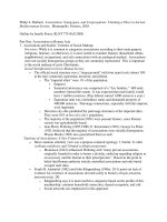
From the survey results, the median of the “General” scores
over all paintings is 3.6, which is selected as the threshold for
labeling images as “low-quality” and “high-quality”, as shown
in the upper histogram of Fig. 8. A painting is labeled as
“low-quality” if its average general score is lower than 3.6. Vice
versa, a painting is labeled as “high-quality” if its average
general score is higher than 3.6. Fig. 7 gives several examples
that are labeled as “high-quality” paintings and “low-quality”
paintings, respectively. What need emphasizing is that these
labels only represent the relative aesthetic quality within the

database and in the eyes of most participants. They are not
judgments given by art-specialists and are not necessarily
relevant with the paintings’ fames or art values.
Only the ‘General’ scores are used in the classification
experiment. The other aspects of scores are used for other
analysis where we got some interesting results. Fig. 8 and Table
II show some statistic data for the human rating scores.
Fig. 8 shows the score distribution. The upper part is a
distribution of the average scores of all the paintings. With the
threshold, the paintings are categorized as “low-quality” or
“high-quality” according to their average score. The bottom part
of Fig. 8 shows the human rating distribution for both categories.
For example, the blue curve shows the ratio of population that
gives a certain score to the paintings that are categorized as


Fig. 8. Score distribution. (a) The upper histogram shows the distribution o
f

the average scores for the 100 paintings. A threshold divides the paintings into
two categories. (b) The bottom graph shows the human rating distributions for
each category, e.g. the blue curve shows the ratio of population that gives a
certain score to the paintings that are categorized as “low-quality” in the upper
histogram.

Fig. 7. Examples that are labeled as “high-quality” and “low-quality” based on
the average scores on them given by human. The paintings on the upper row
are labeled as “high-quality” and those on the bottom row are labeled as
“low-quality”.
> REPLACE THIS LINE WITH YOUR PAPER IDENTIFICATION NUMBER (DOUBLE-CLICK HERE TO EDIT) <

11
“low-quality” due to their average scores. This figure can be
understood on two sides. One side is that the peaks for the two
classes are obviously separated, which confirms the first
assumption for this work – The majority of people tend to have
similar opinions towards many paintings. However, on the other
side, we can also see that there is still a large overlapping region
between the two distributions, which means there is always a
considerate variance in human ratings. This again indicates
what we try to solve is a really subjective problem.
Table II shows the relationship between scores in measure of
different aspects. In this table, each element indicates the
correlation coefficient between the scores for the specific
factors described respectively by the label of that row and the
label of that column.
The correlation coefficients are calculated as below:
Suppose , , ,
GCrCnT
SS S Sare sets of average scores for all
paintings, respectively in the sense of “General”, “Color”,
“Composition” and “Texture”. e.g.
12
[,,,]
NT
GGG G
Sss s= L ,
where
i
G

s
means the average score across users for the
th
i
painting in the sense of “General”.
N is the number of
paintings. Let , , ,
GCrCnT
SS S S
%% % %
be the sets corresponding to the
sets , , ,
GCrCnT
SS S Swith their averages subtracted, e.g.
12
[, ,, ]
NT
GGGGG GG
Sssss ss=− − −
%
L
, where ()
i
GG
s
mean s= . So
the element at position (i, j) of the correlation coefficient matrix
is calculated as:
(:, ) (:, )
_(,)

((:,)) ((:,))
T
ij
Coef mat i j
norm i norm j
⋅
=
⋅
SS
SS

(37)
where
GCrCnT
SS S S
⎡⎤
=
⎣⎦
S
%% % %
.
Since we use the “General” scores for experiment, what we
care most is how the different factors are related to the
“General” scores. It is shown in the first row of Table II, the
three factors to be correlated with the “General” score ranks as
“Composition”, “Color” and “Texture” in descending order.
The high score shows consistency with the questionnaire result
that these three factors are considered important factors for
judging a painting’s aesthetic quality.
IV.

EXPERIMENTS
The aesthetic visual quality assessment work is highly
subjective. Therefore, instead of expecting the computer to give
exact scores on paintings, we simplify the problem into a
two-class problem. That is, to distinguish between paintings
with high aesthetic quality and those with low aesthetic quality.
The classification performance can be measured by the
Receiver Operating Characteristic (ROC) curve, which is
dependent on the False Reject Rate (FRR) and False Accept
Rate (FAR). In this application, the two indicators are
calculated as:
#"" ""
#""
test images with low label but classified as high
FAR
test images with low label
=
(38)
#"" ""
#""
test images with high label but classified as low
FRR
test images with high label
=
(39)
Different pairs of FAR and FRR can be obtained by changing
the decision threshold of a classification method.

A. Classification Methods
Given the set of features, we need to build proper classifier to

combine the features together. Since the metrics based on
different features are not necessarily linear, simple weighted
combination may not work. A straightforward method we use
here is the Naive Bayes Classifier.

1) Naive Bayes Classifier:
Assuming independence between different features and equal
prior probability for both classes, i.e.
12
() ()
P
wPw= , we have:
1111
2222
(|) (|)() (|)
(|) (|)() (|)
P
wX PXwPw PXw
P
wX PXwPw PXw
==
40
1
1
40
2
1
(|)
(| )
i

i
i
i
P
fw
P
fw
=
=
=
∏
∏
(40)
In (39),
X represents the feature vector of a painting
image.
1
w ,
2
w represent the high-quality class and low-quality
class, respectively.
Suppose ( | )
ij
P
fw is coincident with Gaussian distribution,
i.e.
2
(| )~(,())
jj
ij i i

Pf w N
μσ
.
j
i
μ
and
j
i
σ
can be computed in
the training stage. This Gaussian assumption is made only for
simplification. Rationally the distributions for different features
should be considered individually. The Gaussian assumption
may decrease the discriminative ability of some features,
especially those with a distribution containing multiple clusters.
Though unitary Gaussian may not be enough to model the real
distribution of a feature, its two parameters (mean and variance)
do help the classification. For some special case like the hue
harmony model feature, the numerical value used to indicate the
type of a model can be manually selected. Since we found in
training that high-quality paintings tend to fit with the L-type,
I-type, Y-type and X-type better, we assigned consecutive
number (1, 2, 3, 4) for these four models to better satisfy the
Gaussian assumption. Similar implementation is taken for the
S-L model feature. For other features whose numerical values
are automatically computed, we do not make any intervention
on them. Further investigation of modeling feature distribution
and designing classifier is left for future study. In the test stage,
the posterior probability ratio can be computed as Equation (40)

and compared to a threshold in order to make a decision, i.e.
1
1
2
1
2
2
(|)
(|)
(|)
(|)
test
test
Pw X
Tw w
Pw X
Pw X
Tw w
Pw X
⎧
≥⇒ =
⎪
⎪
⎨
⎪
<⇒ =
⎪
⎩

(41)

TABLE II
C
ORRELATIONS BETWEEN SCORES ON DIFFERENT ASPECTS
General Color Composition Texture
General
1.0000 0.8937 0.9160 0.8651
Color 0.8937 1.0000 0.8229 0.8341
Composition 0.9160 0.8229 1.0000 0.8190
Texture 0.8651 0.8341 0.8190 1.0000

> REPLACE THIS LINE WITH YOUR PAPER IDENTIFICATION NUMBER (DOUBLE-CLICK HERE TO EDIT) <

12
By changing the thresholdT , we can get a number of (FAR,
FRR) pairs.
Note here that not all the features are independent, for
example, some features of the largest segment can be correlated
with the global features. Furthermore, the contrast features
between segments may also be highly relevant with the global
contrast. However, the Naive Bayes Method is introduced here
to serve as a baseline classifier, providing a simple but efficient
way to combine the features.

2)
Adaptive Boosting Classifier:
In the Naive Bayes Method, all features are given the same
weight on the final decision. This neglects the fact that some
features may be more powerful while others may be weaker.
Therefore, in order to make better use of the features, we apply
the Adaptive Boosting (AdaBoost) method [18] to adaptively

assign different weights to different features. One feature is
chosen to construct a weak Bayes classifier based on a unitary
Gaussian model.
Finally all the weak classifiers work as a strong classifier,
which can be expressed as:
1
() ()
K
ii i
i
hX h f
α
=
=
∑

(42)
where
{}
|1
i
Xf iK=≤≤, K is the number of weak learners.
()
ii
hx is the corresponding weak classifier to the feature
i
f

and
i

α
is the weight for this weak classifier. So the total number
of weak classifiers equals to the number of features. Therefore,
the decision strategy is:
1
2
()
()
test
test
hX T w w
hX T w w
≥⇒ =
⎧
⎨
<⇒ =
⎩

(43)
Similarly to the previous part, changing the threshold T can
lead to different (FAR, FRR) pairs.
B.
Classification Performance
To evaluate the classification performance, we split the
paintings into two groups as descried in the “Rating Survey” in
Section III. With the ratings from the survey, fifty images are
labeled as “high-quality” and the rest fifty are labeled as
“low-quality”. Since the quantity of images is limited, we adopt
the “leave-N-out” cross validation method for experiment. We
replicate the following course for ten times: From each class, we

randomly select 30 images for training, and 20 for testing. Each
time we lead an independent experiment for training and testing.
In each time’s experiment the threshold T will go through values
between
min max
[, ]TT , with an interval:
max min
TT
T
K
−
Δ=
(44)
K is selected to be 20 in our experiment. For different methods,
min
T and
max
T can be selected differently. The performances for
the each time are recorded and summarized according to the
thresholds after completing the ten-time experiments.
Figures in this section will show the performance of our
proposed approach in different viewpoints.
Fig. 9 gives the overall performance with all the features. The
curves in “red” and “blue” show the average performances in
twenty-time experiments with Naive Bayes classifier and

Fig. 10. Classification performances by using different features
Fig. 9. Performance for the two classification methods

Fig. 11. Classification performances by using different categories of features
> REPLACE THIS LINE WITH YOUR PAPER IDENTIFICATION NUMBER (DOUBLE-CLICK HERE TO EDIT) <

13
TABLE III
I
MPORTANT FEATURES FOR CLASSIFICATION
Feature Meaning of Feature Global / Local
36
f

Brightness contrast between segments Local
10
f

Brightness contrast across the whole image Global
6
f

Hue model the painting fits with Global
11
f

Blurring Effect across the whole image Global
13
f

Horizontal coordinate of the mass center for the
largest segment
Local

39
f

Average saturation for the focus region Local
28
f

Average saturation for the largest segment Local

AdaBoost classifier, respectively. The black line indicating
FAR=1-FRR gives the performance that can be achieved by a
random chance system, which serves as a reference to see how
much better the proposed methods can achieve. We can see that
both Naive Bayes classifier and AdaBoost classifer perform
distinctly better than a random chance system.
Fig. 10 shows classification performances by using different
categories of features. All the results in Fig. 10 are gained
through Naive Bayes Classifier. The red curve indicates the
result by using all the proposed features
{}
|1 40
i
fi≤≤ , while
the other two curves are based on the global features
{}
|1 12
i
fi≤≤ and local features
{}
|13 40

i
fi≤≤ ,
respectively. The global features and the local features achieve
similar performance, respectively. Moreover, combining the
two categories of features can significantly improve the
performance. In Ref [1], only global features are used to assess
photographs. In Ref [2], local features are considered in a
separable way. However, in our work, we not only consider both
global and local features, but also consider the local contrast
between different local parts. The obvious improvement in
performance by combining all features proves that our global
features and local features are complementary.
In Fig. 11, we compare the performance by using features
representing different kind of characteristics. In Table I, we
divide the features into three categories, representing color,
brightness and composition. Some features may relate to more
than one category at the same time. The color features and
composition features perform better than the brightness features.
But we should notice that the brightness group contains fewer
features than the other two and all three groups perform
comparably when the FAR is low.
To look into the role that every individual feature plays, we
study the classification error rates for each weak learner in the
AdaBoost classifier in Fig. 12. The total iteration number for the
AdaBoost classifier is 46 since some features are used more
than once. We can see that the first weak learner has a
26%-round error rate while the 46th weak learner has a
43%-around error rate. Random selection can achieve no larger
than 50% error rate. It tells us that some features may be playing
little roles and it is likely to achieve similar performance by

using fewer features.
Fig. 13 compares classification performance by using
different number of weak learners. This comparison is tested
based on AdaBoost Classifier. Using the top 31 weak learners
can reach similar performance with using all the weak learners.
Those cut-out weak learners may correspond to different
features when using different experiment sets.
We also test the performance for each individual feature by
using Bayes Classifier based on unitary Gaussian model. The
features with the top 10 performance are listed below:
{}
36 13 10 12 28 6 25 39 11 5
,,,,,,,,,
f
fffffffff
Also we can see from the result of the AdaBoost algorithm, the
10 largest weights are assigned to the following features:
{}
36 10 6 11 13 17 32 39 3 28
,,,,,,,,,
f
fffffffff
The above two sets share 7 common features, which play
important roles to the classification in both methods. The
meanings of the seven features are listed in Table III and their
computation methods can be referred to Section II. These
results help us understand further about which features are more
powerful for the aesthetic quality assessment. Fig. 14 gives an

Fig. 12. Classification errors rates for each weak learner in the AdaBoost

Classifier. There are totally 46 weak learners. Some features are selected more
than once since in different iterations training samples are given different
weights and the threshold changes even when using the same feature.

Fig. 13. Classification performances by using different number of weak learners
> REPLACE THIS LINE WITH YOUR PAPER IDENTIFICATION NUMBER (DOUBLE-CLICK HERE TO EDIT) <

14
TABLE IV
C
LASSIFICATION PERFORMANCE OF HUE HISTOGRAM AND HUE MODEL
Methods Classification Error rate
Hue histogram (20-d) + Nearest Neighbor 39.3 %
Hue histogram (20-d) + Naive Bayes 42.0 %
Fitted hue model (1-d) + Bayes 33.8 %

example to show the feature value distribution of the
“Brightness contrast” feature for both classes. We can see that
paintings with high brightness contrast are more likely to be of
high-quality.
We try to explain these results in the following ways, by
connecting with some art knowledge and psychology theory.
1)
36
f
,
10
f
: It is intuitively rational that brightness contrast
affects people’s impression on a painting. The contrast brings

more information than the objects themselves. Large brightness
contrast can create much spatial perception. As said in [7], “All
gradients have the power to create depth, and gradients of
brightness are among the most efficient”.
2)
6
f
: High quality paintings are more likely to fit with these
four models: L-type, I-type, Y-type and X-type, especially the
latter three. The latter three all represent the mixture of
complementary colors. The use of complementary colors is an
important aspect of aesthetically pleasing art and graphic design.
When placed next to each other, complements make each other
appear brighter. When blended the small brushstrokes in
complementary colors together, it creates neutral color and
achieves harmony. We spent a lot of efforts for fitting these
models. Fig. 15 gives an example that this model wins over the
method of simply using the hue histogram. The two paintings
belonging to different quality class have the most similar
histogram. But the models they fit best are different and are
discriminative for the classification. Table IV gives results by
using the two methods.
3)
11
f
: Blurring is sometimes a favorable effect for paintings.
It brings feelings of motion and depth, etc. Professional
photographers try to control the blurring effect at some degree
to keep the moving feel without being too blurred. The result in
our work for this feature is similar. It is likely to be a low-quality

painting when the blurring effect is very large or very small.
4)

13
f
: The relative horizontal coordinate (normalized by the
image width) of the mass center for the largest segment is more
likely to be smaller than 0.5. It can be linked to the “Right and
left” balance in visual psychology. It is discussed in the book [7]
that objects with the size seem to have more weight when put on
the right. So its size needs increasing when put on the left. That
is , larger objects on the left can balance with smaller objects on
the right. It is also said that the important objects are set a bit left
from the center in order to emphasize its importance since a
picture is often read from “left” to “right”.
5)

39
f
,
28
f
: for oil painting, saturation varies due to the
quantity of white pigment mixed in. The saturation for the focus
region tends to be high and that for the largest region tends to be
low for high-quality paintings. Higher saturation is for
emphasizing. However, for large segments, lower saturation
may lead to better harmony and peace.
V.
CONCLUSIONS AND FUTURE WORK

In this paper we proposed a framework to assess the aesthetic
visual quality of paintings. We treat this subjective problem as a
data-driven machine learning problem. We first conduct a
questionnaire survey to study the factors that affect human’s
judgments. Later in a rating survey we have human subjects
score 100 painting images with similar content and in the similar
style. With statistic computation on the rating results, the
paintings are split into two categories relatively with
“high-quality” and “low-quality” labels. Thus the problem is
defined as a two-class classification problem.
To solve the problem, we extract a group of
perception-related features, representing both global


Fig. 14. Brightness contrast feature value distribution for both classes.
Above the histogram, two example paintings belonging to different classes
are shown. The arrows relate the paintings to the zones where their
“Brightness contrast” values lie in.

Fig. 15. Comparison of the discriminability of simple hue histogram and the
hue model. The two paintings are with different quality, but the bottom image
has the most similar hue histogram with that of the upper one. Thus using
only the hue histogram leads to wrong classification. However, the models
they fit with are different. By training, Y-type is favorable for the high-qualit
y

paintings, thus the hue model here works.
> REPLACE THIS LINE WITH YOUR PAPER IDENTIFICATION NUMBER (DOUBLE-CLICK HERE TO EDIT) <

15

TABLE V
D
IRECTIONS FOR THE RATING SURVEY
Please score each image based on your aesthetic visual feeling instead of
judging the art value.

Scores: 1 - 5, 5 means the highest quality while 1 means the lowest quality. A
score is required for the "General" item. For the other items, you could either
give a score or choose "No Concern" to mention you don’t consider the
corresponding property in your decision process.
You are given 25 seconds to look at the paintings. There is a timing bar on
every page. After that, the painting will disappear, but you can still continue
answering the questions on the page. Press the "next" button to score the next
painting when you finish answering the current page.

"General": your whole feeling on this painting at the first sight.
"Color": your feeling on the color present in this painting.
"Composition": your feeling on the organization of objects in the painting.
"Texture": your feeling on the brushstrokes, the marks given to paint by
contact with the bristles of a brush.


characteristics and local characteristics of a painting.
Inspiration for these features comes from our prior knowledge
in art and the criteria mentioned by human subjects in the
questionnaire. These features represent the color, brightness and
composition concepts in a painting. In the classification stage,
two types of classifiers are tested: Naive Bayes classifier and
AdaBoost classifier. Experiments show that both classifiers are
robust to produce good accuracy using the 40 extracted visual

features in discriminating high-rated and low-rated paintings.
Importance of individual feature on the classification
performance is also analyzed, which can help us to decrease the
number of features without significant loss on performance.
This work provides a machine learning scheme for assessing
visual quality in the sense of aesthetics. It aims to explore the
relationship between aesthetic perceptions of human and the
computational visual features extracted from paintings.
Building a connection between human perception on art works
and computational visual features extracted from the art works
is a challenging multidisciplinary problem. Our work is not
meant to provide a full solution, but rather to inspire more
interests in this new and amazing research direction.
Furthermore, the experiment results show that even for such a
subjective problem, with efficient features it is still feasible to
teach the computer to complete the task.
To develop efficient feature metrics is a crucial part for this
research. Although most features extracted here are low-level,
many of them implicitly express important art concepts such as
harmony, balance, complementation, etc. We will keep our
efforts on discovering semantic features in the future. At the
same time, we believe further cooperation with the art
community will provide in-depth vision into the problem. Also,
well-designed psychology survey will assist us to know more
about the tendency in human assessment of paintings, and
further to find related features in the paintings.
Although the assessment is simplified into a two-class
classification task in this work, estimating a quality score for
each painting by regression methods will be part of the future
work. Estimating a quality score can be much helpful for

developing a painting auto-recommendation system.
A
PPENDIX
The complementary details about the survey are given in this
appendix. General introduction has been given in Session III.
The survey includes two parts. Part I is a questionnaire. It is
done before Part II of the survey. 23 subjects participate in the
questionnaire. In this part, subjects are asked to list at least two
factors which are important for them to evaluate the aesthetic
quality of a painting in everyday life. Answers can be ranked
according to their frequency of being mentioned: Color,
Composition /Structure /Form, Meaning /Content, Texture
/Brushstrokes, Shape, Perspective, Feeling of Motion /
Dynamics, Balance, Style, Mood, Originality, Unity, etc.
Part II is a rating survey. We have totally 42 subjects
(including the 23 subjects attending Part I) participate in the
rating survey. None of the participants in the survey are in
art-specialty. Age of the participants varies from 21 to 37. All
of them are with a bachelor’s degree or above and have normal
ability of distinguishing colors. They are asked before the
survey about their preference on painting style. They generally
show neutral feelings on impressionistic style of painting,
neither too enthusiastic nor repulsive.
The rating survey requires each participant to rate at 100
paintings, which are all in the impressionist-style and with the
landscape content. The paintings are downloaded through
“Google image search” with careful selection on size and
definition. The width of the painting images ranges from 768 to
1024 pixels. All paintings are in the JPEG format. Each painting
has an independent rating page. The order of presenting the

paintings to each participant is randomly generated. Table V

Fig. 16. An example page of the survey. When the time decreases to
00:00:00, the painting becomes invisible while the questions remain until
the user clicks the “next” button. The “happy-face” and “unhappy-face” are
used to remind user that higher score corresponds to higher quality.
> REPLACE THIS LINE WITH YOUR PAPER IDENTIFICATION NUMBER (DOUBLE-CLICK HERE TO EDIT) <

16
shows the instructions on a page before the ratings. It directs the
subjects how to rate on the following section and clarifies terms
that are used in the survey.
Fig. 16 shows an example page for rating a painting. A
participant is required to rate a painting in four aspects,
following the rules described in Table V. The participant also
needs to answer whether they know the author of a painting and
whether they feel familiar with a painting. For each painting
used in our experiment, no more than three participants give
“yes” answer to either question. A painting is shown for 25
seconds. After 25 seconds, the painting will disappear. However,
the participant can still complete answering the questions until
he/she presses the “Next” button to go to next painting. This rule
is set to prevent subjects thinking much of the meaning of the
painting. The first sight on a painting is highly related to the
visual perception. As time goes on, human try to combine the
visual feeling with the knowledge in the mind.
A
CKNOWLEDGMENT
The authors thank the volunteers for their participating in the
rating survey and the psychology researchers for providing

strong support for the survey design. The authors also thank all
the anonymous reviewers for their helpful comments and
suggestions.
R
EFERENCES
[1] Yan Ke, Xiaoou Tang, Feng Jing. The Design of High-Level Features for
Photo Quality Assessment. In Proceedings of 2006 IEEE Computer
Society Conference on Computer Vision and Pattern Recognition, vol.
1, pp. 419 – 426.
[2] R. Datta, D. Joshi, J. Li, and J. Z. Wang. Studying aesthetics in
photographic images using a computational approach. Proceedings 2006
European Conference on Computer Vision (ECCV), vol.3, pp. 288-301.
[3] H. Tong, M. Li, H. Zhang, J. He, and C. Zhang. Classification of digital
photos taken by photographers or home users. In Proceedings of Pacific
Rim Conference on Multimedia, 2004.
[4] Ritendra Datta, Jia Li and James Z. Wang "Learning the consensus on
visual quality for next-generation image management," Proceedings of
the ACM Multimedia Conference, pp. 533-536, ACM, Augsburg,
Germany, September 2007.
[5] X. Li. Blind image quality assessment. In Proceedings of International
Conference on Image Processing, 2002.
[6] M. Livingstone, Vision and Art: The Biology of Seeing. Harry N. Abrams,
Inc., Publishers.
[7] R. Arnheim. Art and Visual Perception: a Psychology of the Creative Eye
(expanded and revised edition). University of California Press, 1974.
[8] H. Tong, M. Li, H. Zhang, J. He, and W. Ma. Learning No-reference
Quality Metric by Examples. In Proceedings of International Conference
on Multimedia Modelling, 2005.
[9] Z, Wang, H.R. Sheikh, A.C Bovik, No-reference Perceptual Quality
Assessment of JPEG Compressed Images, in Proceedings of 2002

International Conference on Image Processing. Volume 1, Page(s):I-477
- I-480, 2002.
[10] P. Resnick and H. Varian. Recommender systems. Comm. of the ACM,
40(3):56–58, 1997.
[11] Y. Matusda, Color Design, Asakura Shoten, 1995. (in Japanese).
[12] M. Tokumaru, N. Muranaka, S. Imanishi. Color Design Support System
Considering Color Harmony. In Proceedings of the IEEE International
Conference on Fuzzy Systems, IEEE Press, 378 -383, 2002.
[13] D. Cohen-Or, O. Sorkine, R. Gal, T. Leyvand, Y. Xu. Color
Harmonization, Siggraph 2006.
[14] />
[15] Yuri Boykov, Olga Veksler, Ramin Zabih. Efficient Approximate Energy
Minimization via Graph Cuts, IEEE transactions on PAMI, vol. 20, no. 12,
p. 1222-1239, November 2001.
[16] Vladimir Kolmogorov and Ramin Zabih. What Energy Functions can be
Minimized via Graph Cuts?, IEEE Transactions on PAMI, vol. 26, no. 2,
February 2004, pp. 147-159.
[17] Yuri Boykov and Vladimir Kolmogorov. An Experimental Comparison
of Min-Cut/Max-Flow Algorithms for Energy Minimization in Vision, In
IEEE Transactions on PAMI, vol. 26, no. 9, September 2004, pp.
1124-1137.
[18] Shai Bagon. Matlab Wrapper for Graph Cut, In:
www.wisdom.weizmann.ac.il/~bagon
, December 2006.
[19] Y. Freund and R.E Schapire. Game theory, on-line prediction and
boosting, In Proceedings of the Ninth Annual Conference on
Computational Learning Theory, pages 325-332, 1996.
[20] Johnson, Jr., C. R., E. Hendriks, I. J. Berezhnoy, E. Brevdo, S. M. Hughes,
I. Daubechies, J. Li, E. Postma, and J. Z. Wang, ``Image Processing for
Artist Identification: Computerized Analysis of Vincent van Gogh's

Painting Brushstrokes,'' IEEE Signal Processing Magazine, (Special Issue
on Visual Cultural Heritage), July 2008.
[21] Jia Li and James Z. Wang. Studying Digital Imagery of Ancient Paintings
by Mixtures of Stochastic Models. IEEE Transactions on Image
Processing, vol. 12, no. 2, 15 pp., 2004.
[22] I. E. Berezhnoy, E. O. Postma, and J. van den Herik, Computerized Visual
Analysis of Paintings, Proc. 16th Int. Conf. Assoc. for History and
Computing, pp. 28-32, September 2005.
[23] Shannon Hughes, Eugene Brevdo, and Ingrid Daubechies, Identifying
Hidden Features: A Digital Characterization of Van Gogh's Style,
technical report in Proceedings of the First International Workshop on
Image Processing for Artist Identification, 2007.
[24] D. Rockmore, S. Lyu and H. Farid. A Digital Technique for
Authentication in the Visual Arts, International Foundation for Art
Research, (8)2:12-23, 2006.
[25] I.E. Berezhnoy, E.O. Postma, and H.J. van den Herik. Computer Analysis
of Van Gogh’s Complementary Colours, Pattern Recognition Letters, vol.
28, no. 6, pp. 703 -709, 2007.
[26] D.G. Stork, Computer Vision, Image Analysis, and Master Art: Part 1,
IEEE MultiMedia, vol. 13, no. 3, pp. 16-20, 2006
[27] D.G. Stork and M.K. Johnson, Computer Vision, Image Analysis, and
Master Art, Part 2, IEEE MultiMedia, vol. 13, no. 4, pp. 12-17, 2006.
[28] D.G. Stork and M F. Duarte, Computer Vision, Image Analysis, and
Master Art, Part 3, IEEE Multimedia, vol. 14, no. 1, pp. 14 -18, 2007.
[29] C. M. Falco, Computer Vision and Art, IEEE MultiMedia, vol. 14, no.
2, pp. 8-11, 2007.



Congcong Li is a Ph.D. candidate in Department of Electrical

and Computer Engineering, Carnegie Mellon University,
Pittsburgh, Pennsylvania. She received her B.E. Degree and
M.S. Degree at Department of Electronic Engineering,
Tsinghua University, Beijing, P.R. China, respectively in 2005
and 2007. Her research interests include image processing,
computer vision and pattern recognition.


Tsuhan Chen has been with the School of Electrical and
Computer Engineering, Cornell University, Ithaca, New
York, since January 2009, where he is Professor and
Director. From October 1997 to December 2008, he was
with the Department of Electrical and Computer
Engineering, Carnegie Mellon University, Pittsburgh,
Pennsylvania, as Professor and Associate Department
Head. From August 1993 to October 1997, he worked at
AT&T Bell Laboratories, Holmdel, New Jersey. He
received the M.S. and Ph.D. degrees in electrical engineering from the
California Institute of Technology, Pasadena, California, in 1990 and 1993,
respectively. He received the B.S. degree in electrical engineering from the
National Taiwan University in 1987.
Tsuhan served as the Editor-in-Chief for IEEE Transactions on Multimedia
in 2002-2004. He also served in the Editorial Board of IEEE Signal Processing
Magazine and as Associate Editor for IEEE Trans. on Circuits and Systems for
Video Technology, IEEE Trans. on Image Processing, IEEE Trans. on Signal
Processing, and IEEE Trans. on Multimedia. He co-edited a book titled
Multimedia Systems, Standards, and Networks.
> REPLACE THIS LINE WITH YOUR PAPER IDENTIFICATION NUMBER (DOUBLE-CLICK HERE TO EDIT) <

17

Tsuhan received the Charles Wilts Prize at the California Institute of
Technology in 1993. He was a recipient of the National Science Foundation
CAREER Award, from 2000 to 2003. He received the Benjamin Richard Teare
Teaching Award in 2006, and the Eta Kappa Nu Award for Outstanding
Faculty Teaching in 2007. He was elected to the Board of Governors, IEEE
Signal Processing Society, 2007-2009, and a Distinguished Lecturer, IEEE
Signal Processing Society, 2007-2008. He is a member of the Phi Tau Phi
Scholastic Honor Society, and Fellow of IEEE.