Tài liệu Báo cáo khoa học: "Enhanced word decomposition by calibrating the decision threshold of probabilistic models and using a model ensemble" pdf

Proceedings of the 48th Annual Meeting of the Association for Computational Linguistics, pages 375–383,
Uppsala, Sweden, 11-16 July 2010.
c
2010 Association for Computational Linguistics
Enhanced word decomposition by calibrating the decision threshold of
probabilistic models and using a model ensemble
Sebastian Spiegler
Intelligent Systems Laboratory,
University of Bristol, U.K.

Peter A. Flach
Intelligent Systems Laboratory,
University of Bristol, U.K.

Abstract
This paper demonstrates that the use of
ensemble methods and carefully calibrat-
ing the decision threshold can signifi-
cantly improve the performance of ma-
chine learning methods for morphologi-
cal word decomposition. We employ two
algorithms which come from a family of
generative probabilistic models. The mod-
els consider segment boundaries as hidden
variables and include probabilities for let-
ter transitions within segments. The ad-
vantage of this model family is that it can
learn from small datasets and easily gen-
eralises to larger datasets. The first algo-
rithm PROMODES, which participated in
the Morpho Challenge 2009 (an interna-

tional competition for unsupervised mor-
phological analysis) employs a lower or-
der model whereas the second algorithm
PROMODES-H is a novel development of
the first using a higher order model. We
present the mathematical description for
both algorithms, conduct experiments on
the morphologically rich language Zulu
and compare characteristics of both algo-
rithms based on the experimental results.
1 Introduction
Words are often considered as the smallest unit
of a language when examining the grammatical
structure or the meaning of sentences, referred to
as syntax and semantics, however, words them-
selves possess an internal structure denominated
by the term word morphology. It is worthwhile
studying this internal structure since a language
description using its morphological formation is
more compact and complete than listing all pos-
sible words. This study is called morpholog-
ical analysis. According to Goldsmith (2009)
four tasks are assigned to morphological analy-
sis: word decomposition into morphemes, build-
ing morpheme dictionaries, defining morphosyn-
tactical rules which state how morphemes can
be combined to valid words and defining mor-
phophonological rules that specify phonological
changes morphemes undergo when they are com-
bined to words. Results of morphological analy-

sis are applied in speech synthesis (Sproat, 1996)
and recognition (Hirsimaki et al., 2006), machine
translation (Amtrup, 2003) and information re-
trieval (Kettunen, 2009).
1.1 Background
In the past years, there has been a lot of inter-
est and activity in the development of algorithms
for morphological analysis. All these approaches
have in common that they build a morphologi-
cal model which is then applied to analyse words.
Models are constructed using rule-based meth-
ods (Mooney and Califf, 1996; Muggleton and
Bain, 1999), connectionist methods (Rumelhart
and McClelland, 1986; Gasser, 1994) or statisti-
cal or probabilistic methods (Harris, 1955; Hafer
and Weiss, 1974). Another way of classifying ap-
proaches is based on the learning aspect during
the construction of the morphological model. If
the data for training the model has the same struc-
ture as the desired output of the morphological
analysis, in other words, if a morphological model
is learnt from labelled data, the algorithm is clas-
sified under supervised learning. An example for
a supervised algorithm is given by Oflazer et al.
(2001). If the input data has no information to-
wards the desired output of the analysis, the algo-
rithm uses unsupervised learning. Unsupervised
algorithms for morphological analysis are Lin-
guistica (Goldsmith, 2001), Morfessor (Creutz,
2006) and Paramor (Monson, 2008). Minimally or

semi-supervised algorithms are provided with par-
tial information during the learning process. This
375
has been done, for instance, by Shalonova et al.
(2009) who provided stems in addition to a word
list in order to find multiple pre- and suffixes. A
comparison of different levels of supervision for
morphology learning on Zulu has been carried out
by Spiegler et al. (2008).
Our two algorithms, PROMODES and
PROMODES-H, perform word decomposi-
tion and are based on probabilistic methods
by incorporating a probabilistic generative
model.
1
Their parameters can be estimated
from either labelled data, using maximum like-
lihood estimates, or from unlabelled data by
expectation maximization
2
which makes them
either supervised or unsupervised algorithms.
The purpose of this paper is an analysis of the
underlying probabilistic models and the types of
errors committed by each one. Furthermore, it is
investigated how the decision threshold can be cal-
ibrated and a model ensemble is tested.
The remainder is structured as follows. In Sec-
tion 2 we introduce the probabilistic generative
process and show in Sections 2.1 and 2.2 how

we incorporate this process in PROMODES and
PROMODES-H. We start our experiments with ex-
amining the learning behaviour of the algorithms
in 3.1. Subsequently, we perform a position-wise
comparison of predictions in 3.2, show how we
find a better decision threshold for placing mor-
pheme boundaries in 3.3 and combine both algo-
rithms using a model ensemble to leverage indi-
vidual strengths in 3.4. In 3.5 we examine how
the single algorithms contribute to the result of the
ensemble. In Section 4 we will compare our ap-
proaches to related work and in Section 5 we will
draw our conclusions.
2 Probabilistic generative model
Intuitively, we could say that our models describe
the process of word generation from the left to the
right by alternately using two dice, the first for de-
ciding whether to place a morpheme boundary in
the current word position and the second to get a
corresponding letter transition. We are trying to
reverse this process in order to find the underlying
sequence of tosses which determine the morpheme
boundaries. We are applying the notion of a prob-
1
PROMODES stands for PRObabilistic MOdel for different
DEgrees of Supervision. The H of PROMODES-H refers to
Higher order.
2
In (Spiegler et al., 2009; Spiegler et al., 2010a) we have
presented an unsupervised version of PROMODES.

abilistic generative process consisting of words as
observed variables X and their hidden segmenta-
tion as latent variables Y . If a generative model is
fully parameterised it can be reversed to find the
underlying word decomposition by forming the
conditional probability distribution Pr(Y |X).
Let us first define the model-independent com-
ponents. A given word w
j
∈ W with 1 ≤ j ≤ |W |
consists of n letters and has m = n− 1 positions
for inserting boundaries. A word’s segmentation is
depicted as a boundary vector b
j
= (b
j1
, . ,b
jm
)
consisting of boundary values b
ji
∈ {0, 1} with
1 ≤ i ≤ m which disclose whether or not a bound-
ary is placed in position i. A letter l
j,i-1
precedes
the position i in w
j
and a letter l
ji

follows it. Both
letters l
j,i-1
and l
ji
are part of an alphabet. Fur-
thermore, we introduce a letter transition t
ji
which
goes from l
j,i-1
to l
ji
.
2.1 PROMODES
PROMODES is based on a zero-order model for
boundaries b
ji
and on a first-order model for letter
transitions t
ji
. It describes a word’s segmentation
by its morpheme boundaries and resulting letter
transitions within morphemes. A boundary vector
b
j
is found by evaluating each position i with
argmax
b
ji

Pr(b
ji
|t
ji
) = (1)
argmax
b
ji
Pr(b
ji
)Pr(t
ji
|b
ji
) .
The first component of the equation above is
the probability distribution over non-/boundaries
Pr(b
ji
). We assume that a boundary in i is in-
serted independently from other boundaries (zero-
order) and the graphemic representation of the
word, however, is conditioned on the length of
the word m
j
which means that the probability
distribution is in fact Pr(b
ji
|m
j

). We guarantee
∑
1
r=0
Pr(b
ji
=r|m
j
) = 1. To simplify the notation
in later explanations, we will refer to Pr(b
ji
|m
j
)
as Pr(b
ji
).
The second component is the letter transition
probability distribution Pr(t
ji
|b
ji
). We suppose a
first-order Markov chain consisting of transitions
t
ji
from letter l
j,i-1
∈ A
B

to letter l
ji
∈ A where A
is a regular letter alphabet and A
B
=A ∪{B} in-
cludes B as an abstract morpheme start symbol
which can occur in l
j,i-1
. For instance, the suf-
fix ‘s’ of the verb form gets, marking 3
rd
person
singular, would be modelled as B → s whereas a
morpheme internal transition could be g → e. We
376
guarantee
∑
l
ji
∈A
Pr(t
ji
|b
ji
)=1 with t
ji
being a tran-
sition from a certain l
j,i−1

∈ A
B
to l
ji
. The ad-
vantage of the model is that instead of evaluating
an exponential number of possible segmentations
(2
m
), the best segmentation b
∗
j
=(b
∗
j1
, . ,b
∗
jm
) is
found with 2m position-wise evaluations using
b
∗
ji
= argmax
b
ji
Pr(b
ji
|t
ji

) (2)
=











1, if Pr(b
ji
=1)Pr(t
ji
|b
ji
=1)
> Pr(b
ji
=0)Pr(t
ji
|b
ji
=0)
0, otherwise .
The simplifying assumptions made, however,
reduce the expressive power of the model by not

allowing any dependencies on preceding bound-
aries or letters. This can lead to over-segmentation
and therefore influences the performance of PRO-
MODES. For this reason, we have extended the
model which led to PROMODES-H, a higher-order
probabilistic model.
2.2 PROMODES-H
In contrast to the original PROMODES model, we
also consider the boundary value b
j,i-1
and mod-
ify our transition assumptions for PROMODES-
H in such a way that the new algorithm applies
a first-order boundary model and a second-order
transition model. A transition t
ji
is now defined
as a transition from an abstract symbol in l
j,i-1
∈
{N , B} to a letter in l
ji
∈ A. The abstract sym-
bol is N or B depending on whether b
ji
is 0 or 1.
This holds equivalently for letter transitions t
j,i-1
.
The suffix of our previous example gets would be

modelled N → t → B → s.
Our boundary vector b
j
is then constructed from
argmax
b
ji
Pr(b
ji
|t
ji
,t
j,i-1
, b
j,i-1
) = (3)
argmax
b
ji
Pr(b
ji
|b
j,i-1
)Pr(t
ji
|b
ji
,t
j,i-1
, b

j,i-1
) .
The first component, the probability distribution
over non-/boundaries Pr(b
ji
|b
j,i-1
), satisfies
∑
1
r=0
Pr(b
ji
=r|b
j,i-1
)=1 with b
j,i-1
, b
ji
∈ {0, 1}.
As for PROMODES, Pr(b
ji
|b
j,i-1
) is short-
hand for Pr(b
ji
|b
j,i-1
, m

j
). The second
component, the letter transition proba-
bility distribution Pr(t
ji
|b
ji
, b
j,i-1
), fulfils
∑
l
ji
∈A
Pr(t
ji
|b
ji
,t
j,i-1
, b
j,i-1
)=1 with t
ji
being
a transition from a certain l
j,i−1
∈ A
B
to l

ji
. Once
again, we find the word’s best segmentation b
∗
j
in
2m evaluations with
b
∗
ji
= argmax
b
ji
Pr(b
ji
|t
ji
,t
j,i-1
, b
j,i-1
) = (4)





1, if Pr(b
ji
=1|b

j,i-1
)Pr(t
ji
|b
ji
=1,t
j,i-1
, b
j,i-1
)
> Pr(b
ji
=0|b
j,i-1
)Pr(t
ji
|b
ji
=0,t
j,i-1
, b
j,i-1
)
0, otherwise .
We will show in the experimental results that in-
creasing the memory of the algorithm by looking
at b
j,i−1
leads to a better performance.
3 Experiments and Results

In the Morpho Challenge 2009, PROMODES
achieved competitive results on Finnish, Turkish,
English and German – and scored highest on non-
vowelized and vowelized Arabic compared to 9
other algorithms (Kurimo et al., 2009). For the
experiments described below, we chose the South
African language Zulu since our research work
mainly aims at creating morphological resources
for under-resourced indigenous languages. Zulu
is an agglutinative language with a complex mor-
phology where multiple prefixes and suffixes con-
tribute to a word’s meaning. Nevertheless, it
seems that segment boundaries are more likely in
certain word positions. The PROMODES family
harnesses this characteristic in combination with
describing morphemes by letter transitions. From
the Ukwabelana corpus (Spiegler et al., 2010b) we
sampled 2500 Zulu words with a single segmenta-
tion each.
3.1 Learning with increasing experience
In our first experiment we applied 10-fold cross-
validation on datasets ranging from 500 to 2500
words with the goal of measuring how the learning
improves with increasing experience in terms of
training set size. We want to remind the reader that
our two algorithms are aimed at small datasets.
We randomly split each dataset into 10 subsets
where each subset was a test set and the corre-
sponding 9 remaining sets were merged to a train-
ing set. We kept the labels of the training set

to determine model parameters through maximum
likelihood estimates and applied each model to
the test set from which we had removed the an-
swer keys. We compared results on the test set
against the ground truth by counting true positive
(TP), false positive (FP), true negative (TN) and
377
false negative (FN) morpheme boundary predic-
tions. Counts were summarised using precision
3
,
recall
4
and f-measure
5
, as shown in Table 1.
Data Precision Recall F-measure
500 0.7127±0.0418 0.3500±0.0272 0.4687±0.0284
1000 0.7435±0.0556 0.3350±0.0197 0.4614±0.0250
1500 0.7460±0.0529 0.3160±0.0150 0.4435±0.0206
2000 0.7504±0.0235 0.3068±0.0141 0.4354±0.0168
2500 0.7557±0.0356 0.3045±0.0138 0.4337±0.0163
(a) PROMODES
Data Precision Recall F-measure
500 0.6983±0.0511 0.4938±0.0404 0.5776±0.0395
1000 0.6865±0.0298 0.5177±0.0177 0.5901±0.0205
1500 0.6952±0.0308 0.5376±0.0197 0.6058±0.0173
2000 0.7008±0.0140 0.5316±0.0146 0.6044±0.0110
2500 0.6941±0.0184 0.5396±0.0218 0.6068±0.0151
(b) PROMODES-H

Table 1: 10-fold cross-validation on Zulu.
For PROMODES we can see in Table 1a that
the precision increases slightly from 0.7127 to
0.7557 whereas the recall decreases from 0.3500
to 0.3045 going from dataset size 500 to 2500.
This suggests that to some extent fewer morpheme
boundaries are discovered but the ones which are
found are more likely to be correct. We believe
that this effect is caused by the limited memory
of the model which uses order zero for the occur-
rence of a boundary and order one for letter tran-
sitions. It seems that the model gets quickly sat-
urated in terms of incorporating new information
and therefore precision and recall do not drasti-
cally change for increasing dataset sizes. In Ta-
ble 1b we show results for PROMODES-H. Across
the datasets precision stays comparatively con-
stant around a mean of 0.6949 whereas the recall
increases from 0.4938 to 0.5396. Compared to
PROMODES we observe an increase in recall be-
tween 0.1438 and 0.2351 at a cost of a decrease in
precision between 0.0144 and 0.0616.
Since both algorithms show different behaviour
with increasing experience and PROMODES-H
yields a higher f-measure across all datasets, we
will investigate in the next experiments how these
differences manifest themselves at the boundary
level.
3
precision =

T P
T P+FP
.
4
recall =
T P
T P+FN
.
5
f -measure =
2·precision·recall
precision+recall
.
TN
PH
%=%0.8726%
TN
P
%%%=%0.9472%
%
TP
PH
=%0.5394%
TP
P%%%
=%0.3045%
%
FP
PH
=%0.1274%

FP
P%%%
=%0.0528%
%
%FN
PH%
=%0.4606%
%FN
P%%%%
=%0.6955%
%
0.3109%
0.7889%
0.2111%
0.6891%
+%0.0819%
(net)%
+%0.0486%
(net)%
0.5698%
0.8828%
0.4302%
0.1172%
%
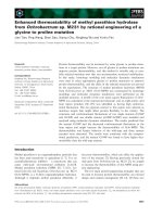
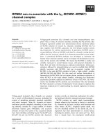
Figure 1: Contingency table for PROMODES [grey
with subscript P] and PROMODES-H [black with
subscript PH] results including gross and net
changes of PROMODES-H.
3.2 Position-wise comparison of algorithmic
predictions

In the second experiment, we investigated which
aspects of PROMODES-H in comparison to PRO-
MODES led to the above described differences in
performance. For this reason we broke down
the summary measures of precision and recall
into their original components: true/false positive
(TP/FP) and negative (TN/FN) counts presented in
the 2 × 2 contingency table of Figure 1. For gen-
eral evidence, we averaged across all experiments
using relative frequencies. Note that the relative
frequencies of positives (TP + FN) and negatives
(TN + FP) each sum to one.
The goal was to find out how predictions
in each word position changed when applying
PROMODES-H instead of PROMODES. This
would show where the algorithms agree and
where they disagree. PROMODES classifies non-
boundaries in 0.9472 of the times correctly as TN
and in 0.0528 of the times falsely as boundaries
(FP). The algorithm correctly labels 0.3045 of the
positions as boundaries (TP) and 0.6955 falsely as
non-boundaries (FN). We can see that PROMODES
follows a rather conservative approach.
When applying PROMODES-H, the majority of
the FP’s are turned into non-boundaries, how-
ever, a slightly higher number of previously cor-
rectly labelled non-boundaries are turned into
false boundaries. The net change is a 0.0486 in-
crease in FP’s which is the reason for the decrease
in precision. On the other side, more false non-

378
boundaries (FN) are turned into boundaries than
in the opposite direction with a net increase of
0.0819 of correct boundaries which led to the in-
creased recall. Since the deduction of precision
is less than the increase of recall, a better over-all
performance of PROMODES-H is achieved.
In summary, PROMODES predicts more accu-
rately non-boundaries whereas PROMODES-H is
better at finding morpheme boundaries. So far we
have based our decision for placing a boundary in
a certain word position on Equation 2 and 4 as-
suming that P(b
ji
=1|. ) > P(b
ji
=0|. )
6
gives the
best result. However, if the underlying distribu-
tion for boundaries given the evidence is skewed,
it might be possible to improve results by introduc-
ing a certain decision threshold for inserting mor-
pheme boundaries. We will put this idea to the test
in the following section.
3.3 Calibration of the decision threshold
For the third experiment we slightly changed our
experimental setup. Instead of dividing datasets
during 10-fold cross-validation into training and
test subsets with the ratio of 9:1 we randomly split

the data into training, validation and test sets with
the ratio of 8:1:1. We then run our experiments
and measured contingency table counts.
Rather than placing a boundary if
P(b
ji
=1|. ) > P(b
ji
=0|. ) which corresponds
to P(b
ji
=1|. ) > 0.50 we introduced a decision
threshold P(b
ji
=1|. ) > h with 0 ≤ h ≤ 1. This
is based on the assumption that the underlying
distribution P(b
ji
|. ) might be skewed and an
optimal decision can be achieved at a different
threshold. The optimal threshold was sought on
the validation set and evaluated on the test set.
An overview over the validation and test results
is given in Table 2. We want to point out that the
threshold which yields the best f-measure result
on the validation set returns almost the same
result on the separate test set for both algorithms
which suggests the existence of a general optimal
threshold.
Since this experiment provided us with a set of

data points where the recall varied monotonically
with the threshold and the precision changed ac-
cordingly, we reverted to precision-recall curves
(PR curves) from machine learning. Following
Davis and Goadrich (2006) the algorithmic perfor-
6
Based on Equation 2 and 4 we use the notation P(b
ji
|. . .)
if we do not want to specify the algorithm.
mance can be analysed more informatively using
these kinds of curves. The PR curve is plotted with
recall on the x-axis and precision on the y-axis for
increasing thresholds h. The PR curves for PRO-
MODES and PROMODES-H are shown in Figure
2 on the validation set from which we learnt our
optimal thresholds h
∗
. Points were connected for
readability only – points on the PR curve cannot
be interpolated linearly.
In addition to the PR curves, we plotted isomet-
rics for corresponding f-measure values which are
defined as precision=
f -measure·recall
2recall−f -measure
and are hy-
perboles. For increasing f-measure values the iso-
metrics are moving further to the top-right corner
of the plot. For a threshold of h = 0.50 (marked

by ‘✸’) PROMODES-H has a better performance
than PROMODES. Nevertheless, across the entire
PR curve none of the algorithms dominates. One
curve would dominate another if all data points
of the dominated curve were beneath or equal
to the dominating one. PROMODES has its opti-
mal threshold at h
∗
= 0.36 and PROMODES-H at
h
∗
= 0.37 where PROMODES has a slightly higher
f-measure than PROMODES-H. The points of op-
timal f-measure performance are marked with ‘’
on the PR curve.
Prec. Recall F-meas.
PROMODES validation (h=0.50) 0.7522 0.3087 0.4378
PROMODES test (h=0.50) 0.7540 0.3084 0.4378
PROMODES validation (h
∗
=0.36) 0.5857 0.7824 0.6699
PROMODES test (h
∗
=0.36) 0.5869 0.7803 0.6699
PROMODES-H validation (h=0.50) 0.6983 0.5333 0.6047
PROMODES-H test (h=0.50) 0.6960 0.5319 0.6030
PROMODES-H validation (h
∗
=0.37) 0.5848 0.7491 0.6568
PROMODES-H test (h

∗
=0.37) 0.5857 0.7491 0.6574
Table 2: PROMODES and PROMODES-H on vali-
dation and test set.
Summarizing, we have shown that both algo-
rithms commit different errors at the word posi-
tion level whereas PROMODES is better in pre-
dicting non-boundaries and PROMODES-H gives
better results for morpheme boundaries at the de-
fault threshold of h = 0.50. In this section, we
demonstrated that across different decision thresh-
olds h for P(b
ji
=1|. ) > h none of algorithms
dominates the other one, and at the optimal thresh-
old PROMODES achieves a slightly higher perfor-
mance than PROMODES-H. The question which
arises is whether we can combine PROMODES and
PROMODES-H in an ensemble that leverages indi-
vidual strengths of both.
379
0.4 0.5 0.6 0.7 0.8 0.9 1
0.4
0.5
0.6
0.7
0.8
0.9
1
Recall

Precision


Promodes
Promodes−H
Promodes−E
F−measure isometrics
Default result
Optimal result (h*)
Figure 2: Precision-recall curves for algorithms on validation set.
3.4 A model ensemble to leverage individual
strengths
A model ensemble is a set of individually trained
classifiers whose predictions are combined when
classifying new instances (Opitz and Maclin,
1999). The idea is that by combining PROMODES
and PROMODES-H, we would be able to avoid cer-
tain errors each model commits by consulting the
other model as well. We introduce PROMODES-E
as the ensemble of PROMODES and PROMODES-
H. PROMODES-E accesses the individual proba-
bilities Pr(b
ji
=1|. ) and simply averages them:
Pr(b
ji
=1|t
ji
) +Pr(b
ji

=1|t
ji
, b
j,i-1
,t
j,i-1
)
2
> h .
As before, we used the default threshold
h = 0.50 and found the calibrated threshold
h
∗
= 0.38, marked with ‘✸’ and ‘’ in Figure 2
and shown in Table 3. The calibrated threshold
improves the f-measure over both PROMODES and
PROMODES-H.
Prec. Recall F-meas.
PROMODES-E validation (h=0.50) 0.8445 0.4328 0.5723
PROMODES-E test (h=0.50) 0.8438 0.4352 0.5742
PROMODES-E validation (h
∗
=0.38) 0.6354 0.7625 0.6931
PROMODES-E test (h
∗
=0.38) 0.6350 0.7620 0.6927
Table 3: PROMODES-E on validation and test set.
The optimal solution applying h
∗
= 0.38 is

more balanced between precision and recall and
boosted the original result by 0.1185 on the test
set. Compared to its components PROMODES and
PROMODES-H the f-measure increased by 0.0228
and 0.0353 on the test set.
In short, we have shown that by combining
PROMODES and PROMODES-H and finding the
optimal threshold, the ensemble PROMODES-E
gives better results than the individual models
themselves and therefore manages to leverage the
individual strengths of both to a certain extend.
However, can we pinpoint the exact contribution
of each individual algorithm to the improved re-
sult? We try to find an answer to this question in
the analysis of the subsequent section.
3.5 Analysis of calibrated algorithms and
their model ensemble
For the entire dataset of 2500 words, we have
examined boundary predictions dependent on the
relative word position. In Figure 3 and 4 we have
plotted the absolute counts of correct boundaries
(TP) and non-boundaries (TN) which PROMODES
predicted but not PROMODES-H, and vice versa,
as continuous lines. We furthermore provided the
number of individual predictions which were ulti-
mately adopted by PROMODES-E in the ensemble
as dashed lines.
In Figure 3a we can see for the default thresh-
old that PROMODES performs better in predicting
non-boundaries in the middle and the end of the

word in comparison to PROMODES-H. Figure 3b
380
shows the statistics for correctly predicted bound-
aries. Here, PROMODES-H outperforms PRO-
MODES in predicting correct boundaries across the
entire word length. After the calibration, shown
in Figure 4a, PROMODES-H improves the correct
prediction of non-boundaries at the beginning of
the word whereas PROMODES performs better at
the end. For the boundary prediction in Figure 4b
the signal disappears after calibration.
Concluding, it appears that our test language
Zulu has certain features which are modelled best
with either a lower or higher-order model. There-
fore, the ensemble leveraged strengths of both al-
gorithms which led to a better overall performance
with a calibrated threshold.
4 Related work
We have presented two probabilistic genera-
tive models for word decomposition, PROMODES
and PROMODES-H. Another generative model
for morphological analysis has been described
by Snover and Brent (2001) and Snover et al.
(2002), however, they were interested in finding
paradigms as sets of mutual exclusive operations
on a word form whereas we are describing a gener-
ative process using morpheme boundaries and re-
sulting letter transitions.
Moreover, our probabilistic models seem to re-
semble Hidden Markov Models (HMMs) by hav-

ing certain states and transitions. The main differ-
ence is that we have dependencies between states
as well as between emissions whereas in HMMs
emissions only depend on the underlying state.
Combining different morphological analysers
has been performed, for example, by Atwell and
Roberts (2006) and Spiegler et al. (2009). Their
approaches, though, used majority vote to decide
whether a morpheme boundary is inserted in a cer-
tain word position or not. The algorithms them-
selves were treated as black-boxes.
Monson et al. (2009) described an indirect
approach to probabilistically combine ParaMor
(Monson, 2008) and Morfessor (Creutz, 2006).
They used a natural language tagger which was
trained on the output of ParaMor and Morfes-
sor. The goal was to mimic each algorithm since
ParaMor is rule-based and there is no access to
Morfessor’s internally used probabilities. The tag-
ger would then return a probability for starting a
new morpheme in a certain position based on the
original algorithm. These probabilities in com-
bination with a threshold, learnt on a different
dataset, were used to merge word analyses. In
contrast, our ensemble algorithm PROMODES-E
directly accesses the probabilistic framework of
each algorithm and combines them based on an
optimal threshold learnt on a validation set.
5 Conclusions
We have presented a method to learn a cali-

brated decision threshold from a validation set and
demonstrated that ensemble methods in connec-
tion with calibrated decision thresholds can give
better results than the individual models them-
selves. We introduced two algorithms for word de-
composition which are based on generative prob-
abilistic models. The models consider segment
boundaries as hidden variables and include prob-
abilities for letter transitions within segments.
PROMODES contains a lower order model whereas
PROMODES-H is a novel development of PRO-
MODES with a higher order model. For both
algorithms, we defined the mathematical model
and performed experiments on language data of
the morphologically complex language Zulu. We
compared the performance on increasing train-
ing set sizes and analysed for each word position
whether their boundary prediction agreed or dis-
agreed. We found out that PROMODES was bet-
ter in predicting non-boundaries and PROMODES-
H gave better results for morpheme boundaries at
a default decision threshold. At an optimal de-
cision threshold, however, both yielded a simi-
lar f-measure result. We then performed a fur-
ther analysis based on relative word positions and
found out that the calibrated PROMODES-H pre-
dicted non-boundaries better for initial word posi-
tions whereas the calibrated PROMODES for mid-
and final word positions. For boundaries, the cali-
brated algorithms had a similar behaviour. Subse-

quently, we showed that a model ensemble of both
algorithms in conjunction with finding an optimal
threshold exceeded the performance of the single
algorithms at their individually optimal threshold.
Acknowledgements
We would like to thank Narayanan Edakunni and
Bruno Gol
´
enia for discussions concerning this pa-
per as well as the anonymous reviewers for their
comments. The research described was sponsored
by EPSRC grant EP/E010857/1 Learning the mor-
phology of complex synthetic languages.
381
0.1 0.2 0.3 0.4 0.5 0.6 0.7 0.8 0.9 1
0
100
200
300
400
500
600
700
800
Relative word position
Absolute true negatives (TN)
Performance on non−boundaries, default threshold


Promodes (unique TN)

Promodes−H (unique TN)
Promodes and Promodes−E (unique TN)
Promodes−H and Promodes−E (unique TN)
(a) True negatives, default
0.1 0.2 0.3 0.4 0.5 0.6 0.7 0.8 0.9 1
0
100
200
300
400
500
600
700
800
Relative word position
Absolute true positives (TP)
Performance on boundaries, default threshold


Promodes (unique TP)
Promodes−H (unique TP)
Promodes and Promodes−E (unique TP)
Promodes−H and Promodes−E (unique TP)
(b) True positives, default
Figure 3: Analysis of results using default threshold.
0.1 0.2 0.3 0.4 0.5 0.6 0.7 0.8 0.9 1
0
100
200
300

400
500
600
700
800
Relative word position
Absolute true negatives (TN)
Performance on non−boundaries, calibrated threshold


Promodes (unique TN)
Promodes−H (unique TN)
Promodes and Promodes−E (unique TN)
Promodes−H and Promodes−E (unique TN)
(a) True negatives, calibrated
0.1 0.2 0.3 0.4 0.5 0.6 0.7 0.8 0.9 1
0
100
200
300
400
500
600
700
800
Relative word position
Absolute true positives (TP)
Performance on boundaries, calibrated threshold

Promodes (unique TP)
Promodes−H (unique TP)
Promodes and Promodes−E (unique TP)
Promodes−H and Promodes−E (unique TP)
(b) True positives, calibrated
Figure 4: Analysis of results using calibrated threshold.
382
References
J. W. Amtrup. 2003. Morphology in machine trans-
lation systems: Efficient integration of finite state
transducers and feature structure descriptions. Ma-
chine Translation, 18(3):217–238.
E. Atwell and A. Roberts. 2006. Combinatory hy-
brid elementary analysis of text (CHEAT). Proceed-
ings of the PASCAL Challenges Workshop on Un-
supervised Segmentation of Words into Morphemes,
Venice, Italy.
M. Creutz. 2006. Induction of the Morphology of Nat-
ural Language: Unsupervised Morpheme Segmen-
tation with Application to Automatic Speech Recog-
nition. Ph.D. thesis, Helsinki University of Technol-
ogy, Espoo, Finland.
J. Davis and M. Goadrich. 2006. The relationship
between precision-recall and ROC curves. Interna-
tional Conference on Machine Learning, Pittsburgh,
PA, 233–240.
M. Gasser. 1994. Modularity in a connectionist
model of morphology acquisition. Proceedings of
the 15th conference on Computational linguistics,
1:214–220.

J. Goldsmith. 2001. Unsupervised learning of the mor-
phology of a natural language. Computational Lin-
guistics, 27:153–198.
J. Goldsmith. 2009. The Handbook of Computational
Linguistics, chapter Segmentation and morphology.
Blackwell.
M. A. Hafer and S. F. Weiss. 1974. Word segmenta-
tion by letter successor varieties. Information Stor-
age and Retrieval, 10:371–385.
Z. S. Harris. 1955. From phoneme to morpheme. Lan-
guage, 31(2):190–222.
T. Hirsimaki, M. Creutz, V. Siivola, M. Kurimo, S. Vir-
pioja, and J. Pylkkonen. 2006. Unlimited vocabu-
lary speech recognition with morph language mod-
els applied to Finnish. Computer Speech And Lan-
guage, 20(4):515–541.
K. Kettunen. 2009. Reductive and generative ap-
proaches to management of morphological variation
of keywords in monolingual information retrieval:
An overview. Journal of Documentation, 65:267 –
290.
M. Kurimo, S. Virpioja, and V. T. Turunen. 2009.
Overview and results of Morpho Challenge 2009.
Working notes for the CLEF 2009 Workshop, Corfu,
Greece.
C. Monson, K. Hollingshead, and B. Roark. 2009.
Probabilistic ParaMor. Working notes for the CLEF
2009 Workshop, Corfu, Greece.
C. Monson. 2008. ParaMor: From Paradigm
Structure To Natural Language Morphology Induc-

tion. Ph.D. thesis, Language Technologies Institute,
School of Computer Science, Carnegie Mellon Uni-
versity, Pittsburgh, PA, USA.
R. J. Mooney and M. E. Califf. 1996. Learning the
past tense of English verbs using inductive logic pro-
gramming. Symbolic, Connectionist, and Statistical
Approaches to Learning for Natural Language Pro-
cessing, 370–384.
S. Muggleton and M. Bain. 1999. Analogical predic-
tion. Inductive Logic Programming: 9th Interna-
tional Workshop, ILP-99, Bled, Slovenia, 234.
K. Oflazer, S. Nirenburg, and M. McShane. 2001.
Bootstrapping morphological analyzers by combin-
ing human elicitation and machine learning. Com-
putational. Linguistics, 27(1):59–85.
D. Opitz and R. Maclin. 1999. Popular ensemble
methods: An empirical study. Journal of Artificial
Intelligence Research, 11:169–198.
D. E. Rumelhart and J. L. McClelland. 1986. On
learning the past tenses of English verbs. MIT
Press, Cambridge, MA, USA.
K. Shalonova, B. Gol
´
enia, and P. A. Flach. 2009. To-
wards learning morphology for under-resourced fu-
sional and agglutinating languages. IEEE Transac-
tions on Audio, Speech, and Language Processing,
17(5):956965.
M. G. Snover and M. R. Brent. 2001. A Bayesian
model for morpheme and paradigm identification.

Proceedings of the 39th Annual Meeting on Asso-
ciation for Computational Linguistics, 490 – 498.
M. G. Snover, G. E. Jarosz, and M. R. Brent. 2002.
Unsupervised learning of morphology using a novel
directed search algorithm: Taking the first step. Pro-
ceedings of the ACL-02 workshop on Morphological
and phonological learning, 6:11–20.
S. Spiegler, B. Gol
´
enia, K. Shalonova, P. A. Flach, and
R. Tucker. 2008. Learning the morphology of Zulu
with different degrees of supervision. IEEE Work-
shop on Spoken Language Technology.
S. Spiegler, B. Gol
´
enia, and P. A. Flach. 2009. Pro-
modes: A probabilistic generative model for word
decomposition. Working Notes for the CLEF 2009
Workshop, Corfu, Greece.
S. Spiegler, B. Gol
´
enia, and P. A. Flach. 2010a. Un-
supervised word decomposition with the Promodes
algorithm. In Multilingual Information Access Eval-
uation Vol. I, CLEF 2009, Corfu, Greece, Lecture
Notes in Computer Science, Springer.
S. Spiegler, A. v. d. Spuy, and P. A. Flach. 2010b. Uk-
wabelana - An open-source morphological Zulu cor-
pus. in review.
R. Sproat. 1996. Multilingual text analysis for text-to-

speech synthesis. Nat. Lang. Eng., 2(4):369–380.
383