Tài liệu Báo cáo khoa học: "Untangling the Cross-Lingual Link Structure of Wikipedia" pptx
Bạn đang xem bản rút gọn của tài liệu. Xem và tải ngay bản đầy đủ của tài liệu tại đây (336.12 KB, 10 trang )
Proceedings of the 48th Annual Meeting of the Association for Computational Linguistics, pages 844–853,
Uppsala, Sweden, 11-16 July 2010.
c
2010 Association for Computational Linguistics
Untangling the Cross-Lingual Link Structure of Wikipedia
Gerard de Melo
Max Planck Institute for Informatics
Saarbr
¨
ucken, Germany
Gerhard Weikum
Max Planck Institute for Informatics
Saarbr
¨
ucken, Germany
Abstract
Wikipedia articles in different languages
are connected by interwiki links that are
increasingly being recognized as a valu-
able source of cross-lingual information.
Unfortunately, large numbers of links are
imprecise or simply wrong. In this pa-
per, techniques to detect such problems are
identified. We formalize their removal as
an optimization task based on graph re-
pair operations. We then present an al-
gorithm with provable properties that uses
linear programming and a region growing
technique to tackle this challenge. This
allows us to transform Wikipedia into a
much more consistent multilingual regis-
ter of the world’s entities and concepts.
1 Introduction
Motivation. The open community-maintained en-
cyclopedia Wikipedia has not only turned the In-
ternet into a more useful and linguistically di-
verse source of information, but is also increas-
ingly being used in computational applications as
a large-scale source of linguistic and encyclope-
dic knowledge. To allow cross-lingual navigation,
Wikipedia offers cross-lingual interwiki links that
for instance connect the Indonesian article about
Albert Einstein to the corresponding articles in
over 100 other languages. Such links are extraor-
dinarily valuable for cross-lingual applications.
In the ideal case, a set of articles connected di-
rectly or indirectly via such links would all de-
scribe the same entity or concept. Due to concep-
tual drift, different granularities, as well as mis-
takes made by editors, we frequently find con-
cepts as different as economics and manager in the
same connected component. Filtering out inaccu-
rate links enables us to exploit Wikipedia’s multi-
linguality in a much safer manner and allows us to
create a multilingual register of named entities.
Contribution. Our research contributions are:
1) We identify criteria to detect inaccurate connec-
tions in Wikipedia’s cross-lingual link structure.
2) We formalize the task of removing such links
as an optimization problem. 3) We introduce an
algorithm that attempts to repair the cross-lingual
graph in a minimally invasive way. This algorithm
has an approximation guarantee with respect to
optimal solutions. 4) We show how this algorithm
can be used to combine all editions of Wikipedia
into a single large-scale multilingual register of
named entities and concepts.
2 Detecting Inaccurate Links
In this paper, we model the union of cross-lingual
links provided by all editions of Wikipedia as an
undirected graph G = (V, E) with edge weights
w(e) for e ∈ E. In our experiments, we simply
honour each individual link equally by defining
w(e) = 2 if there are reciprocal links between the
two pages, 1 if there is a single link, and 0 other-
wise. However, our framework is flexible enough
to deal with more advanced weighting schemes,
e.g. one could easily plug in cross-lingual mea-
sures of semantic relatedness between article texts.
It turns out that an astonishing number of con-
nected components in this graph harbour inac-
curate links between articles. For instance, the
Esperanto article ‘Germana Imperiestro’ is about
German emporers and another Esperanto article
‘Germana Imperiestra Regno’ is about the Ger-
man Empire, but, as of June 2010, both are linked
to the English and German articles about the Ger-
man Empire. Over time, some inaccurate links
may be fixed, but in this and in large numbers of
other cases, the imprecise connection has persisted
for many years. In order to detect such cases, we
need to have some way of specifying that two ar-
ticles are likely to be distinct.
844
Figure 1: Connected component with inaccurate
links (simplified)
2.1 Distinctness Assertions
Figure 1 shows a connected component that con-
flates the concept of television as a medium with
the concept of TV sets as devices. Among other
things, we would like to state that ‘Television’ and
‘T.V.’ are distinct from ‘Television set’ and ‘TV
set’. In general, we may have several sets of enti-
ties D
i,1
, . . . , D
i,l
i
, for which we assume that any
two entities u,v from different sets are pairwise
distinct with some degree of confidence or weight.
In our example, D
i,1
= {‘Television’,‘T.V.’}
would be one set, and D
i,2
= {‘Television set’,‘TV
set’} would be another set, which means that we
are assuming ‘Television’, for example, to be dis-
tinct from both ‘Television set’ and ‘TV set’.
Definition 1. (Distinctness Assertions) Given a
set of nodes V , a distinctness assertion is a col-
lection D
i
= (D
i,1
, . . . , D
i,l
i
) of pairwise dis-
joint (i.e. D
i,j
∩ D
i,k
= ∅ for j = k) sub-
sets D
i,j
⊂ V that expresses that any two nodes
u ∈ D
i,j
, v ∈ D
i,k
from different subsets (j = k)
are asserted to be distinct from each other with
some weight w(D
i
) ∈ R.
We found that many components with inaccurate
links can be identified automatically with the fol-
lowing distinctness assertions.
Criterion 1. (Distinctness between articles from
the same Wikipedia edition) For each language-
specific edition of Wikipedia, a separate asser-
tion (D
i,1
, D
i,2
, . . . ) can be made, where each
D
i,j
contains an individual article together with
its respective redirection pages. Two articles from
the same Wikipedia very likely describe distinct
concepts unless they are redirects of each other.
For example, ‘Georgia (country)’ is distinct from
‘Georgia (U.S. State)’. Additionally, there are also
redirects that are clearly marked by a category or
template as involving topic drift, e.g. redirects
from songs to albums or artists, from products to
companies, etc. We keep such redirects in a D
i,j
distinct from the one of their redirect targets.
Criterion 2. (Distinctness between categories
from the same Wikipedia edition) For each
language-specific edition of Wikipedia, a separate
assertion (D
i,1
, D
i,2
, . . . ) is made, where each
D
i,j
contains a category page together with any
redirects. For instance, ‘Category:Writers’ is dis-
tinct from ‘Category:Writing’.
Criterion 3. (Distinctness for links with anchor
identifiers) The English ‘Division by zero’, for in-
stance, links to the German ‘Null#Division’. The
latter is only a part of a larger article about the
number zero in general, so we can make a dis-
tinctness assertion to separate ‘Division by zero’
from ‘Null’. In general, for each interwiki link or
redirection with an anchor identifier, we add an as-
sertion (D
i,1
, D
i,2
) where D
i,1
,D
i,2
represent the
respective articles without anchor identifiers.
These three types of distinctness assertions are
instantiated for all articles and categories of all
Wikipedia editions. The assertion weights are tun-
able; the simplest choice is using a uniform weight
for all assertions (note that these weights are dif-
ferent from the edge weights in the graph). We
will revisit this issue in our experiments.
2.2 Enforcing Consistency
Given a graph G representing cross-lingual links
between Wikipedia pages, as well as distinctness
assertions D
1
, . . . , D
n
with weights w(D
i
), we
may find that nodes that are asserted to be dis-
tinct are in the same connected component. We
can then try to apply repair operations to recon-
cile the graph’s link structure with the distinctness
asssertions and obtain global consistency. There
are two ways to modify the input, and for each
we can also consider the corresponding weights
as a sort of cost that quantifies how much we are
changing the original input:
a) Edge cutting: We may remove an edge e ∈
E from the graph, paying cost w(e).
b) Distinctness assertion relaxation: We may
remove a node v ∈ V from a distinctness as-
sertion D
i
, paying cost w(D
i
).
845
Removing edges allows us to split connected com-
ponents into multiple smaller components, thereby
ensuring that two nodes asserted to be distinct are
no longer connected directly or indirectly. In Fig-
ure 1, for instance, we could delete the edge from
the Spanish ‘TV set’ article to the Japanese ‘televi-
sion’ article. In constrast, removing nodes from
distinctness assertions means that we decide to
give up our claim of them being distinct, instead
allowing them to share a connected component.
Our reliance on costs is based on the assump-
tion that the link structure or topology of the graph
provides the best indication of which cross-lingual
links to remove. In Figure 1, we have distinct-
ness assertions between nodes in two densely con-
nected clusters that are tied together only by a sin-
gle spurious link. In such cases, edge removals
can easily yield separate connected components.
When, however, the two nodes are strongly con-
nected via many different paths with high weights,
we may instead opt for removing one of the two
nodes from the distinctness assertion.
The aim will be to balance the costs for remov-
ing edges from the graph with the costs for remov-
ing nodes from distinctness assertions to produce
a consistent solution with a minimal total repair
cost. We accommodate our knowledge about dis-
tinctness while staying as close as possible to what
Wikipedia provides as input.
This can be formalized as the Weighted
Distinctness-Based Graph Separation (WDGS)
problem. Let G be an undirected graph with a set
of vertices V and a set of edges E weighted by
w : E → R. If we use a set C ⊆ V to spec-
ify which edges we want to cut from the original
graph, and sets U
i
to specify which nodes we want
to remove from distinctness assertions, we can be-
gin by defining WDGS solutions as follows.
Definition 2. (WDGS Solution). Given a graph
G = (V, E) and n distinctness assertions D
1
, . . . ,
D
n
, a tuple (C, U
1
, . . . , U
n
) is a valid WDGS so-
lution if and only if ∀i, j, k = j, u ∈ D
i,j
\ U
i
,
v ∈ D
i,k
\ U
i
: P(u, v, E \ C) = ∅, i.e. the set of
paths from u to v in the graph (V, E \ C) is empty.
Definition 3. (WDGS Cost). Let w : E → R
be a weight function for edges e ∈ E, and w(D
i
)
(i = 1 . . . n) be weights for the distinctness as-
sertions. The (total) cost of a WDGS solution
S = (C, U
1
, . . . , U
n
) is then defined as
c(S) = c(C, U
1
, . . . , U
n
)
=
e∈C
w(e)
+
n
i=1
|U
i
| w(D
i
)
Definition 4. (WDGS). A WDGS problem instance
P consists of a graph G = (V, E) with edge
weights w(e) and n distinctness assertions D
1
,
. . . , D
n
with weights w(D
i
). The objective con-
sists in finding a solution (C, U
1
, . . . , U
n
) with
minimal cost c(C, U
1
, . . . , U
n
).
It turns out that finding optimal solutions effi-
ciently is a hard problem (proofs in Appendix A).
Theorem 1. WDGS is NP-hard and APX-hard. If
the Unique Games Conjecture (Khot, 2002) holds,
then it is NP-hard to approximate WDGS within
any constant factor α > 0.
3 Approximation Algorithm
Due to the hardness of WDGS, we devise a
polynomial-time approximation algorithm with an
approximation factor of 4 ln(nq + 1) where n is
the number of distinctness assertions and q =
max
i,j
|D
i,j
|. This means that for all problem in-
stances P , we can guarantee
c(S(P ))
c(S
∗
(P ))
≤ 4 ln(nq + 1),
where S(P ) is the solution determined by our al-
gorithm, and S
∗
(P ) is an optimal solution. Note
that this approximation guarantee is independent
of how long each D
i
is, and that it merely repre-
sents an upper bound on the worst case scenario.
In practice, the results tend to be much closer to
the optimum, as will be shown in Section 4.
Our algorithm first solves a linear program (LP)
relaxation of the original problem, which gives
us hints as to which edges should most likely be
cut and which nodes should most likely be re-
moved from distinctness assertions. Note that this
is a continuous LP, not an integer linear program
(ILP); the latter would not be tractable due to the
large number of variables and constraints of the
problem. After solving the linear program, a new
– extended – graph is constructed and the optimal
LP solution is used to define a distance metric on
it. The final solution is obtained by smartly se-
lecting regions in this extended graph as the in-
dividual output components, employing a region
846
growing technique in the spirit of the seminal work
by Leighton and Rao (1999). Edges that cross the
boundaries of these regions are cut.
Definition 5. Given a WDGS instance, we define a
linear program of the following form:
minimize
e∈E
d
e
w(e) +
n
i=1
l
i
j=1
v∈D
i,j
u
i,v
w(D
i
)
subject to
p
i,j,v
= u
i,v
∀i, j<l
i
, v ∈ D
i,j
(1)
p
i,j,v
+ u
i,v
≥ 1 ∀i, j<l
i
, v ∈
S
k>j
D
i,k
(2)
p
i,j,v
≤ p
i,j,u
+ d
e
∀i, j<l
i
, e=(u,v) ∈ E (3)
d
e
≥ 0 ∀e ∈ E (4)
u
i,v
≥ 0 ∀i, v ∈
l
i
S
j=1
D
i,j
(5)
p
i,j,v
≥ 0 ∀i, j<l
i
, v∈V (6)
The LP uses decision variables d
e
and u
i,v
, and
auxiliary variables p
i,j,v
that we refer to as poten-
tial variables. The d
e
variables indicate whether
(in the continuous LP: to what degree) an edge
e should be deleted, and the u
i,v
variables indi-
cate whether (to what degree) v should be removed
from a distinctness assertion D
i
. The LP objec-
tive function corresponds to Definition 3, aiming
to minimize the total costs. A potential variable
p
i,j,v
reflects a sort of potential difference between
an assertion D
i,j
and a node v. If p
i,j,v
= 0, then v
is still connected to nodes in D
i,j
. Constraints (1)
and (2) enforce potential differences between D
i,j
and all nodes in D
i,k
with k > j. For instance,
for distinctness between ‘New York City’ and ‘New
York’ (the state), they might require ‘New York’
to have a potential of 1, while ‘New York City’
has a potential of 0. The potential variables are
tied to the deletion variables d
e
for edges in Con-
straint (3) as well as to the u
i,v
in Constraints (1)
and (2). This means that the potential difference
p
i,j,v
+ u
i,v
≥ 1 can only be obtained if edges are
deleted on every path between ‘New York City’ and
‘New York’, or if at least one of these two nodes is
removed from the distinctness assertion (by setting
the corresponding u
i,v
to non-zero values). Con-
straints (4), (5), (6) ensure non-negativity.
Having solved the linear program, the next ma-
jor step is to convert the optimal LP solution into
the final – discrete – solution. We cannot rely
on standard rounding methods to turn the optimal
fractional values of the d
e
and u
i,v
variables into
a valid solution. Often, all solution variables have
small values and rounding will merely produce an
empty (C, U
1
, . . . , U
n
) = (∅, ∅, . . . , ∅). Instead,
a more sophisticated technique is necessary. The
optimal solution of the LP can be used to define
an extended graph G
with a distance metric d be-
tween nodes. The algorithm then operates on this
graph, in each iteration selecting regions that be-
come output components and removing them from
the graph. A simple example is shown in Figure 2.
The extended graph contains additional nodes and
edges representing distinctness assertions. Cutting
one of these additional edges corresponds to re-
moving a node from a distinctness assertion.
Definition 6. Given G = (V, E) and distinct-
ness assertions D
1
, . . . , D
n
with weights w(D
i
),
we define an undirected graph G
= (V
, E
)
where V
= V ∪ {v
i,v
| i = 1 . . . n, w(D
i
) >
0, v ∈
j
D
i,j
}, E
= {e ∈ E | w(e) > 0} ∪
{(v, v
i,v
) | v ∈ D
i,j
, w(D
i
) > 0}. We accordingly
extend the definition of w(e) to additionally cover
the new edges by defining w(e) = w(D
i
) for e =
(v, v
i,v
). We also extend it for sets S of edges by
defining w(S) =
e∈S
w(e). Finally, we define a
node distance metric
d(u, v) =
0 u = v
d
e
(u, v) ∈ E
u
i,v
u = v
i,v
u
i,u
v = v
i,u
min
p∈
P(u,v,E
)
(u
,v
)
∈p
d(u
, v
) otherwise,
where P(u, v, E
) denotes the set of acyclic paths
between two nodes in E
. We further fix
ˆc
f
=
(u,v)∈E
d(u, v) w(e)
as the weight of the fractional solution of the LP
(ˆc
f
is a constant based on the original E
, irre-
spective of later modifications to the graph).
Definition 7. Around a given node v in G
, we
consider regions R(v, r) ⊆ V with radius r. The
cut C(v, r) of a given region is defined as the set
of edges in G
with one endpoint within the region
and one outside the region:
R(v, r) = {v
∈ V
| d(v, v
) ≤ r}
C(v, r) = {e ∈ E
| |e ∩ R(v, r)| = 1}
For sets of nodes S ⊆ V , we define R(S, r) =
v∈S
R(v, r) and C(S, r) =
v∈S
C(v, r).
847
Figure 2: Extended graph with two added nodes
v
1,u
, v
1,v
representing distinctness between ‘Tele-
visi
´
on’ and ‘Televisor’, and a region around v
1,u
that would cut the link from the Japanese ‘Televi-
sion’ to ‘Televisor’
Definition 8. Given q = max
i,j
|D
i,j
|, we approxi-
mate the optimal cost of regions as:
ˆc(v, r) =
e=(u,u
)∈E
:
e⊆R(v,r)
d(u, u
) w(e) (1)
+
e∈C(v,r)
v
∈e∩R(v,r)
(r − d(v, v
)) w(e)
ˆc(S, r) =
1
nq
ˆc
f
+
v∈S
ˆc(v, r) (2)
The first summand accounts for the edges en-
tirely within the region, and the second one ac-
counts for the edges in C(v, r) to the extent that
they are within the radius. The definition of ˆc(S, r)
contains an additional slack component that is re-
quired for the approximation guarantee proof.
Based on these definitions, Algorithm 3.1 uses
the LP solution to construct the extended graph.
It then repeatedly, as long as there is an unsatis-
fied assertion D
i
, chooses a set S of nodes con-
taining one node from each relevant D
i,j
. Around
the nodes in S it simultaneously grows |S| regions
with the same radius, a technique previously sug-
gested by Avidor and Langberg (2007). These re-
gions are essentially output components that de-
termine the solution. Repeatedly choosing the
radius that minimizes
w(C(S,r))
ˆc(S,r)
allows us to ob-
tain the approximation guarantee, because the dis-
tances in this extended graph are based on the so-
lution of the LP. The properties of this algorithm
are given by the following two theorems (proofs in
Appendix A).
Theorem 2. The algorithm yields a valid WDGS
solution (C, U
1
, . . . , U
n
).
Theorem 3. The algorithm yields a solution
(C, U
1
, . . . , U
n
) with an approximation factor of
4 ln(nq + 1) with respect to the cost of the op-
timal WDGS solution (C
∗
, U
∗
1
, . . . , U
∗
n
), where n
is the number of distinctness assertions and q =
max
i,j
|D
i,j
|. This solution can be obtained in poly-
nomial time.
4 Results
4.1 Wikipedia
We downloaded February 2010 XML dumps of
all available editions of Wikipedia, in total 272
editions that amount to 86.5 GB uncompressed.
From these dumps we produced two datasets.
Dataset A captures cross-lingual interwiki links
between pages, in total 77.07 million undirected
edges (146.76 million original links). Dataset
B additionally includes 2.2 million redirect-based
edges. Wikipedia deals with interwiki links to
redirects transparently, however there are many
redirects with titles that do not co-refer, e.g. redi-
rects from members of a band to the band, or from
aspects of a topic to the topic in general. We only
included redirects in the following cases:
• the titles of redirect and redirect target match
after Unicode NFKD normalization, diacrit-
ics removal, case conversion, and removal of
punctuation characters
• the redirect uses certain templates or cate-
gories that indicate co-reference with the tar-
get (alternative names, abbreviations, etc.)
We treated them like reciprocal interwiki links by
assigning them a weight of 2.
4.2 Application of Algorithm
The choice of distinctness assertion weights de-
pends on how lenient we wish to be towards con-
ceptual drift, allowing us to opt for more fine- or
more coarse-grained distinctions. In our experi-
ments, we decided to prefer fine-grained concep-
tual distinctions, and settled on a weight of 100.
We analysed over 20 million connected com-
ponents in each dataset, checking for distinctness
assertions. For the roughly 110,000 connected
components with relevant distinctness assertions,
848
Algorithm 3.1 WDGS Approximation Algorithm
1: procedure SELECT(V, E, V
, E
, w, D
1
, . . . , D
n
, l
1
, . . . , l
n
)
2: solve linear program given by Definition 5 determine optimal fractional solution
3: construct G
= (V
, E
) extended graph (Definition 6)
4: C ← {e ∈ E | w(e) = 0} cut zero-weighted edges
5: U
i
←
l
i
−1
j=1
D
i,j
∀i : w(D
i
) = 0 remove zero-weighted D
i
6: while ∃i, j, k > j, u ∈ D
i,j
, v ∈ D
i,k
: P(v
i,u
, v
i,v
, E
) = ∅ do find unsatisfied assertion
7: S ← ∅ set of nodes around which regions will be grown
8: for all j in 1 . . . l
i
− 1 do arbitrarily choose node from each D
i,j
9: if ∃v ∈ D
i,j
: v
i,v
∈ V
then S ← S ∪ v
i,v
10: D ← {d(u, v) ≤
1
2
| u ∈ S, v ∈ V
} ∪ {
1
2
} set of distances
11: choose such that ∀d, d
∈ D : 0 < |d − d
| infinitesimally small
12: r ← argmin
r=d−: d∈D\{0}
w(C(S, r))
ˆc(S, r)
choose optimal radius (ties broken arbitrarily)
13: V
← V
\ R(S, r) remove regions from G
14: E
← {e ∈ E
| e ⊆ V
}
15: C ← C ∪ (C(S, r) ∩ E) update global solution
16: for all i
in 1 . . . n do
17: U
i
← U
i
∪ {v | (v
i
,v
, v) ∈ C(S, r)}
18: for all j in 1 . . . l
i
do D
i
,j
← D
i
,j
∩ V
prune distinctness assertions
19: return (C, U
1
, . . . , U
n
)
we applied our algorithm, relying on the commer-
cial CPLEX tool to solve the linear programs. In
most cases, the LP solving took less than a second,
however the LP sizes grow exponentially with the
number of nodes and hence the time complex-
ity increases similarly. In about 300 cases per
dataset, CPLEX took too long and was automat-
ically killed or the linear program was a priori
deemed too large to complete in a short amount
of time. For these cases, we adopted an alternative
strategy described later on.
Table 1 provides the experimental results for the
two datasets. Dataset B is more connected and
thus has fewer connected components with more
pairs of nodes asserted to be distinct by distinct-
ness assertions. The LP given by Definition 5
provides fractional solutions that constitute lower
bounds on the optimal solution (cf. also Lemma
5 in Appendix A), so the optimal solution can-
not have a cost lower than the fractional LP solu-
tion. Table 1 shows that in practice, our algorithm
achieves near-optimal results.
4.3 Linguistic Adequacy
The near-optimal results of our algorithm apply
with respect to our problem formalization, which
aims at repairing the graph in a minimally inva-
Table 1: Algorithm Results
Dataset A Dataset B
Connected
components
23,356,027 21,161,631
– with distinctness
assertions
112,857 113,714
– algorithm applied
successfully
112,580 113,387
Distinctness
assertions
380,694 379,724
Node pairs con-
sidered distinct
916,554 1,047,299
Lower bound on
optimal cost
1,255,111 1,245,004
Cost of our solution 1,306,747 1,294,196
Factor 1.04 1.04
Edges to be deleted
(undirected)
1,209,798 1,199,181
Nodes to be merged 603 573
sive way. It may happen, however, that the graph’s
topology is misleading, and that in a specific case
deleting many cross-lingual links to separate two
entities is more appropriate than looking for a
conservative way to separate them. This led us
849
to study the linguistic adequacy. Two annotators
evaluated 200 randomly selected separated pairs
from Dataset A consisting of an English and a
German article, with an inter-annotator agreement
(Cohen κ) of 0.656. Examples are given in Table
2. We obtained a precision of 87.97% ± 0.04%
(Wilson score interval) against the consensus an-
notation. Many of the errors are the result of ar-
ticles having many inaccurate outgoing links, in
which case they may be assigned to the wrong
component. In other cases, we noted duplicate ar-
ticles in Wikipedia.
Occasionally, we also observed differences in
scope, where one article would actually describe
two related concepts in a single page. Our algo-
rithm will then either make a somewhat arbitrary
assignment to the component of either the first or
second concept, or the broader generalization of
the two concepts becomes a separate, more gen-
eral connected component.
4.4 Large Problem Instances
When problem instances become too large, the lin-
ear programs can become too unwieldy for lin-
ear optimization software to cope with on current
hardware. In such cases, the graphs tend to be very
sparsely connected, consisting of many smaller,
more densely connected subgraphs. We thus in-
vestigated graph partitioning heuristics to decom-
pose larger graphs into smaller parts that can more
easily be handled with our algorithm. The METIS
algorithms (Karypis and Kumar, 1998) can de-
compose graphs with hundreds of thousands of
nodes almost instantly, but favour equally sized
clusters over lower cut costs. We obtained parti-
tionings with costs orders of magnitude lower us-
ing the heuristic by Dhillon et al. (2007).
4.5 Database of Named Entities
The partitioning heuristics allowed us to process
all entries in the complete set of Wikipedia dumps
and produce a clean output set of connected com-
ponents where each Wikipedia article or category
belongs to a connected component consisting of
pages about the same entity or concept. We can re-
gard these connected components as equivalence
classes. This means that we obtain a large-scale
multilingual database of named entities and their
translations. We are also able to more safely trans-
fer information cross-lingually between editions.
For example, when an article a has a category c in
the French Wikipedia, we can suggest the corre-
sponding Indonesian category for the correspond-
ing Indonesian article.
Moreover, we believe that this database will
help extend resources like DBPedia and YAGO
that to date have exclusively used the English
Wikipedia as their repository of entities and
classes. With YAGO’s category heuristics, even
entirely non-English connected components can
be assigned a class in WordNet as long as at least
one of the relevant categories has an English page.
So, the French Wikipedia article on the Dutch
schooner ‘JR Tolkien’, despite the lack of a cor-
responding English article, can be assigned to the
WordNet synset for ‘ship’. Using YAGO’s plu-
ral heuristic to distinguish classes (Einstein is a
physicist) from topic descriptors (Einstein belongs
to the topic physics), we determined that over 4.8
million connected components can be linked to
WordNet, greatly surpassing the 3.2 million arti-
cles covered by the English Wikipedia alone.
5 Related Work
A number of projects have used Wikipedia as a
database of named entities (Ponzetto and Strube,
2007; Silberer et al., 2008). The most well-
known are probably DBpedia (Auer et al., 2007),
which serves as a hub in the Linked Data Web,
Freebase
1
, which combines human input and au-
tomatic extractors, and YAGO (Suchanek et al.,
2007), which adds an ontological structure on top
of Wikipedia’s entities. Wikipedia has been used
cross-lingually for cross-lingual IR (Nguyen et al.,
2009), question answering (Ferr
´
andez et al., 2007)
as well as for learning transliterations (Pasternack
and Roth, 2009), among other things.
Mihalcea and Csomai (2007) have studied pre-
dicting new links within a single edition of
Wikipedia. Sorg and Cimiano (2008) considered
the problem of suggesting new cross-lingual links,
which could be used as additional inputs in our
problem. Adar et al. (2009) and Bouma et al.
(2009) show how cross-lingual links can be used
to propagate information from one Wikipedia’s in-
foboxes to another edition.
Our aggregation consistency algorithm uses
theoretical ideas put forward by researchers study-
ing graph cuts (Leighton and Rao, 1999; Garg et
al., 1996; Avidor and Langberg, 2007). Our prob-
lem setting is related to that of correlation cluster-
ing (Bansal et al., 2004), where a graph consist-
1
/>850
Table 2: Examples of separated concepts
English concept German concept
(translated)
Explanation
Coffee percolator French Press different types of brewing devices
Baqa-Jatt Baqa al-Gharbiyye Baqa-Jatt is a city resulting from a merger
of Baqa al-Gharbiyye and Jatt
Leucothoe (plant) Leucothea (Orchamos) the second refers to a figure of Greek
mythology
Old Belarusian language Ruthenian language the second is often considered slightly
broader
ing of positively and negatively labelled similar-
ity edges is clustered such that similar items are
grouped together, however our approach is much
more generic than conventional correlation clus-
tering. Charikar et al. (2005) studied a variation
of correlation clustering that is similar to WDGS,
but since a negative edge would have to be added
between each relevant pair of entities in a distinct-
ness assertion, the approximation guarantee would
only be O(log(n |V |
2
)). Minimally invasive re-
pair operations on graphs have also been stud-
ied for graph similarity computation (Zeng et al.,
2009), where two graphs are provided as input.
6 Conclusions and Future Work
We have presented an algorithmic framework for
the problem of co-reference that produces consis-
tent partitions by intelligently removing edges or
allowing nodes to remain connected. This algo-
rithm has successfully been applied to Wikipedia’s
cross-lingual graph, where we identified and elim-
inated surprisingly large numbers of inaccurate
connections, leading to a large-scale multilingual
register of names.
In future work, we would like to investigate
how our algorithm behaves in extended settings,
e.g. we can use heuristics to connect isolated,
unconnected articles to likely candidates in other
Wikipedias using weighted edges. This can be
extended to include mappings from multiple lan-
guages to WordNet synsets, with the hope that
the weights and link structure will then allow the
algorithm to make the final disambiguation deci-
sion. Additional scenarios include dealing with
co-reference on the Linked Data Web or mappings
between thesauri. As such resources are increas-
ingly being linked to Wikipedia and DBpedia, we
believe that our techniques will prove useful in
making mappings more consistent.
A Proofs
Proof (Theorem 1). We shall reduce the mini-
mum multicut problem to WDGS. The hardness
claims then follow from Chawla et al. (2005).
Given a graph G = (V, E) with a positive cost
c(e) for each e ∈ E, and a set D = {(s
i
, t
i
) | i =
1 . . . k} of k demand pairs, our goal is to find
a multicut M with respect to D with minimum
total cost
e∈M
c(e). We convert each demand
pair (s
i
, t
i
) into a distinctness assertion D
i
=
({s
i
}, {t
i
}) with weight w(D
i
) = 1+
e∈E
c(e).
An optimal WDGS solution (C, U
1
, . . . , U
k
) with
cost c then implies a multicut C with the same
weight, because each w(D
i
) >
e∈E
c(e), so
all demand pairs will be satisfied. C is a minimal
multicut because any multicut C
with lower cost
would imply a valid WDGS solution (C
, ∅, . . . , ∅)
with a cost lower than the optimal one, which is a
contradiction.
Lemma 4. The linear program given by Defini-
tion 5 enforces that for any i,j,k = j,u ∈ D
i,j
,
v ∈ D
i,k
, and any path v
0
, . . . , v
t
with v
0
= u,
v
t
= v we obtain u
i,u
+
t−1
l=0
d
(v
l
,v
l+1
)
+u
i,v
≥ 1.
The integer linear program obtained by aug-
menting Definition 5 with integer constraints
d
e
, u
i,v
, p
i,j,v
∈ {0, 1} (for all applicable e, i, j,
v) produces optimal solutions (C, U
1
, . . . , U
k
) for
WDGS problems, obtained as C = ({e ∈ E | d
e
=
1}, U
i
= {v | u
i,v
= 1}.
Proof. Without loss of generality, let us assume
that j < k. The LP constraints give us p
i,j,v
t
≤
p
i,j,v
t−1
+d
(v
t−1
,v
t
)
, . . . , p
i,j,v
1
≤ p
i,j,v
0
+d
(v
0
,v
1
)
,
as well as p
i,j,v
0
= u
i,u
and p
i,j,v
t
+ u
i,v
≥ 1.
Hence 1 ≤ p
i,j,v
t
+u
i,v
≤ u
i,u
+
t−1
l=0
d
(v
l
,v
l+1
)
+
u
i,v
.
With added integrality constraints, we obtain ei-
ther u ∈ U
i
, v ∈ U
i
, or at least one edge along any
path from u to v is cut, i.e. P(u, v, E \ C) = ∅.
851
This proves that any ILP solution enduces a valid
WDGS solution (Definition 2).
Clearly, the integer program’s objective func-
tion minimizes c(C, U
1
, . . . , U
n
) (Definition 3) if
C = ({e ∈ E | d
e
= 1}, U
i
= {v | u
i,v
= 1}.
To see that the solutions are optimal, it thus suf-
fices to observe that any optimal WDGS solution
(C
∗
, U
∗
1
, . . . , U
∗
n
) yields a feasible ILP solution
d
e
= I
C
∗
(e), u
i,v
= I
U
∗
i
(v).
Proof (Theorem 2). r
i
<
1
2
holds for any ra-
dius r
i
chosen by the algorithm, so for any re-
gion R(v
0
, r) grown around a node v
0
, and any
two nodes u, v within that region, the triangle in-
equality gives us d(u, v) ≤ d(u, v
0
) + d(v
0
, v) <
1
2
+
1
2
= 1 (maximal distance condition). At
the same time, by Lemma 4 and Definition 6 for
any u ∈ D
i,j
, v ∈ D
i,k
(j = k), we obtain
d(v
i,u
, v
i,v
) = d(v
i,u
, u) + d(u, v) + d(v, v
i,v
) ≥
1. With the maximal distance condition above, this
means that v
i,u
and v
i,v
cannot be in the same re-
gion. Hence u, v cannot be in the same region,
unless the edge from v
i,u
to u is cut (in which case
u will be placed in U
i
) or the edge from v to v
i,v
is cut (in which case v will be placed in U
i
). Since
each region is separated from other regions via C,
we obtain that ∀i, j, k = j, u, v: u ∈ D
i,j
\ U
i
,
v ∈ D
i,k
\ U
i
implies P(u, v, E \ C) = ∅, so a
valid solution is obtained.
Lemma 5 (essentially due to Garg et al. (1996)).
For any i where ∃j, k > j, u ∈ D
i,j
, v ∈ D
i,k
:
P(v
i,u
, v
i,v
, E
) = ∅ and w(D
i
) > 0, there exists
an r such that w(C(S, r)) ≤ 2 ln(nq + 1) ˆc(S, r),
0 ≤ r <
1
2
for any set S consisting of v
i,v
nodes.
Proof. Define w(S, r) =
v∈S
w(C(v, r)). We
will prove that there exists an appropriate r with
w(C(S, r)) ≤ w(S, r) ≤ 2 ln(nq+1) ˆc(S, r). As-
sume, for reductio ad absurdum, that ∀r ∈ [0,
1
2
) :
w(S, r) > 2 ln(nq + 1)ˆc(S, r). As we expand
the radius r, we note that ˆc(S, r)
d
dr
= w(S, r)
whereever ˆc is differentiable with respect to r.
There are only a finite number of points r
1
,. . . ,r
l−1
in (0,
1
2
) where this is not the case (namely, when
∃u ∈ S, v ∈ V
: d(u, v) = r
i
). Also note
that ˆc increases monotonically for increasing val-
ues of r, and that it is universally greater than
zero (since there is a path between v
i,u
, v
i,v
). Set
r
0
= 0, r
l
=
1
2
and choose such that 0 <
min{r
j+1
− r
j
| j < l}. Our assumption then
implies:
l
j=1
r
j
−
r
j−1
+
w(S,r)
ˆc(S,r)
dr
>
l
j=1
r
j
− r
j−1
− 2
2 ln(nq + 1)
l
j=1
ln ˆc(S, r
j
− ) − ln ˆc(S, r
j−1
+ )
>
1
2
− 2l
2 ln(nq + 1)
ln ˆc(S,
1
2
− ) − ln ˆc(S, 0)
> (1 − 4l) ln(nq + 1)
ˆc(S,
1
2
−)
ˆc(S,0)
> (nq + 1)
1−4l
ˆc(S,
1
2
− ) > (nq + 1)
1−4l
ˆc(S, 0)
For small , the right term can get arbitrarily close
to (nq + 1)ˆc(S, 0) ≥ ˆc
f
+ ˆc(S, 0), which is strictly
larger than ˆc(S,
1
2
− ) no matter how small be-
comes, so the initial assumption is false.
Proof (Theorem 3). Let S
i
, r
i
denote the set
S and radius r chosen in particular iterations,
and c
i
the corresponding costs incurred: c
i
=
w(C(S
i
, r) ∩ E) + |U
i
|w(D
i
) = w(C(D
i
, r)).
Note that any r
i
chosen by the algorithm will in
fact fulfil the criterion described by Lemma 5, be-
cause r
i
is chosen to minimize the ratio between
the two terms, and the minimizing r ∈ [0,
1
2
)
must be among the r considered by the algo-
rithm (w(C(D
i
, r)) only changes at one of those
points, so the minimum is reached by approach-
ing the points from the left). Hence, we obtain
c
i
≤ 2 ln(n + 1)ˆc(S
i
, r
i
). For our global solution,
note that there is no overlap between the regions
chosen within an iteration, since regions have a
radius strictly smaller than
1
2
, while v
i,u
, v
i,v
for
u ∈ D
i,j
, v ∈ D
i,k
, j = k have a distance of
at least 1. Nor is there any overlap between re-
gions from different iterations, because in each it-
eration the selected regions are removed from G
.
Globally, we therefore obtain c(C, U
1
, . . . , U
n
) =
i
c
i
< 2 ln(nq + 1)
i
ˆc(S
i
, r
i
) ≤ 2 ln(nq +
1)2ˆc
f
(observe that i ≤ nq). Since ˆc
f
is the ob-
jective score for the fractional LP relaxation solu-
tion of the WDGS ILP (Lemma 4), we obtain ˆc
f
≤
c(C
∗
, U
∗
1
, . . . , U
∗
n
), and thus c(C, U
1
, . . . , U
n
) <
4 ln(n + 1)c(C
∗
, U
∗
1
, . . . , U
∗
n
).
To obtain a solution in polynomial time, note
that the LP size is polynomial with respect to nq
and may be solved using a polynomial algorithm
(Karmarkar, 1984). The subsequent steps run in
O(nq) iterations, each growing up to |V | regions
using O(|V |
2
) uniform cost searches.
852
References
Eytan Adar, Michael Skinner, and Daniel S. Weld.
2009. Information arbitrage across multi-lingual
Wikipedia. In Ricardo A. Baeza-Yates, Paolo Boldi,
Berthier A. Ribeiro-Neto, and Berkant Barla Cam-
bazoglu, editors, Proceedings of the 2nd Interna-
tional Conference on Web Search and Web Data
Mining, WSDM 2009, pages 94–103. ACM.
S
¨
oren Auer, Chris Bizer, Jens Lehmann, Georgi Kobi-
larov, Richard Cyganiak, and Zachary Ives. 2007.
DBpedia: a nucleus for a web of open data. In
Aberer et al., editor, The Semantic Web, 6th Interna-
tional Semantic Web Conference, 2nd Asian Seman-
tic Web Conference, ISWC 2007 + ASWC 2007, Bu-
san, Korea, November 11–15, 2007, Lecture Notes
in Computer Science 4825. Springer.
Adi Avidor and Michael Langberg. 2007. The multi-
multiway cut problem. Theoretical Computer Sci-
ence, 377(1-3):35–42.
Nikhil Bansal, Avrim Blum, and Shuchi Chawla. 2004.
Correlation clustering. Machine Learning, 56(1-
3):89–113.
Gosse Bouma, Sergio Duarte, and Zahurul Islam.
2009. Cross-lingual alignment and completion of
Wikipedia templates. In CLIAWS3 ’09: Proceed-
ings of the Third International Workshop on Cross
Lingual Information Access, pages 21–29, Morris-
town, NJ, USA. Association for Computational Lin-
guistics.
Moses Charikar, Venkatesan Guruswami, and Anthony
Wirth. 2005. Clustering with qualitative informa-
tion. Journal of Computer and System Sciences,
71(3):360–383.
Shuchi Chawla, Robert Krauthgamer, Ravi Kumar, Yu-
val Rabani, and D. Sivakumar. 2005. On the hard-
ness of approximating multicut and sparsest-cut. In
In Proceedings of the 20th Annual IEEE Conference
on Computational Complexity, pages 144–153.
Inderjit S. Dhillon, Yuqiang Guan, and Brian Kulis.
2007. Weighted graph cuts without eigenvectors.
a multilevel approach. IEEE Trans. Pattern Anal.
Mach. Intell., 29(11):1944–1957.
Sergio Ferr
´
andez, Antonio Toral,
´
Oscar Ferr
´
andez, An-
tonio Ferr
´
andez, and Rafael Mu
˜
noz. 2007. Ap-
plying Wikipedia’s multilingual knowledge to cross-
lingual question answering. In NLDB, pages 352–
363.
Naveen Garg, Vijay V. Vazirani, and Mihalis Yan-
nakakis. 1996. Approximate max-flow min-
(multi)cut theorems and their applications. SIAM
Journal on Computing (SICOMP), 25:698–707.
Narendra Karmarkar. 1984. A new polynomial-time
algorithm for linear programming. In STOC ’84:
Proceedings of the 16th Annual ACM Symposium on
Theory of Computing, pages 302–311, New York,
NY, USA. ACM.
George Karypis and Vipin Kumar. 1998. A fast and
high quality multilevel scheme for partitioning irreg-
ular graphs. SIAM Journal on Scientific Computing,
20(1):359–392.
Subhash Khot. 2002. On the power of unique 2-prover
1-round games. In STOC ’02: Proceedings of the
34th Annual ACM Symposium on Theory of Com-
puting, pages 767–775, New York, NY, USA. ACM.
Tom Leighton and Satish Rao. 1999. Multicommodity
max-flow min-cut theorems and their use in design-
ing approximation algorithms. Journal of the ACM,
46(6):787–832.
Rada Mihalcea and Andras Csomai. 2007. Wikify!:
Linking documents to encyclopedic knowledge. In
Proceedings of the 16th ACM Conference on Infor-
mation and Knowledge Management (CIKM 2007),
pages 233–242, New York, NY, USA. ACM.
D. Nguyen, A. Overwijk, C. Hauff, R.B. Trieschnigg,
D. Hiemstra, and F.M.G. Jong de. 2009. Wiki-
Translate: query translation for cross-lingual infor-
mation retrieval using only Wikipedia. In Carol
Peters, Thomas Deselaers, Nicola Ferro, and Julio
Gonzalo, editors, Evaluating Systems for Multilin-
gual and Multimodal Information Access, Lecture
Notes in Computer Science 5706, pages 58–65.
Jeff Pasternack and Dan Roth. 2009. Learning bet-
ter transliterations. In CIKM ’09: Proceeding of the
18th ACM Conference on Information and Knowl-
edge Management, pages 177–186, New York, NY,
USA. ACM.
Simone Paolo Ponzetto and Michael Strube. 2007. De-
riving a large scale taxonomy from Wikipedia. In
AAAI 2007: Proceedings of the 22nd Conference
on Artificial Intelligence, pages 1440–1445. AAAI
Press.
Carina Silberer, Wolodja Wentland, Johannes Knopp,
and Matthias Hartung. 2008. Building a multilin-
gual lexical resource for named entity disambigua-
tion, translation and transliteration. In European,
editor, Proceedings of the Sixth International Lan-
guage Resources and Evaluation (LREC’08), Mar-
rakech, Morocco.
Philipp Sorg and Philipp Cimiano. 2008. Enrich-
ing the crosslingual link structure of Wikipedia - a
classification-based approach. In Proceedings of the
AAAI 2008 Workshop on Wikipedia and Artifical In-
telligence.
Fabian M. Suchanek, Gjergji Kasneci, and Gerhard
Weikum. 2007. Yago: A Core of Semantic Knowl-
edge. In Proceedings of the 16th International
World Wide Web conference, WWW, New York, NY,
USA. ACM Press.
Zhiping Zeng, Anthony K. H. Tung, Jianyong Wang,
Jianhua Feng, and Lizhu Zhou. 2009. Comparing
stars: On approximating graph edit distance. Pro-
ceedings of the VLDB Endowment, 2(1):25–36.
853