Tài liệu Báo cáo khoa học: "k-best Spanning Tree Parsing" pptx
Bạn đang xem bản rút gọn của tài liệu. Xem và tải ngay bản đầy đủ của tài liệu tại đây (229.57 KB, 8 trang )
Proceedings of the 45th Annual Meeting of the Association of Computational Linguistics, pages 392–399,
Prague, Czech Republic, June 2007.
c
2007 Association for Computational Linguistics
k-best Spanning Tree Parsing
Keith Hall
Center for Language and Speech Processing
Johns Hopkins University
Baltimore, MD 21218
keith
Abstract
This paper introduces a Maximum Entropy
dependency parser based on an efficient k-
best Maximum Spanning Tree (MST) algo-
rithm. Although recent work suggests that
the edge-factored constraints of the MST al-
gorithm significantly inhibit parsing accu-
racy, we show that generating the 50-best
parses according to an edge-factored model
has an oracle performance well above the
1-best performance of the best dependency
parsers. This motivates our parsing ap-
proach, which is based on reranking the k-
best parses generated by an edge-factored
model. Oracle parse accuracy results are
presented for the edge-factored model and
1-best results for the reranker on eight lan-
guages (seven from CoNLL-X and English).
1 Introduction
The Maximum Spanning Tree algorithm
1
was re-
cently introduced as a viable solution for non-
projective dependency parsing (McDonald et al.,
2005b). The dependency parsing problem is nat-
urally a spanning tree problem; however, effi-
cient spanning-tree optimization algorithms assume
a cost function which assigns scores independently
to edges of the graph. In dependency parsing, this
effectively constrains the set of models to those
which independently generate parent-child pairs;
1
In this paper we deal only with MSTs on directed graphs.
These are often referred to in the graph-theory literature as Max-
imum Spanning Arborescences.
these are known as edge-factored models. These
models are limited to relatively simple features
which exclude linguistic constructs such as verb
sub-categorization/valency, lexical selectional pref-
erences, etc.
2
In order to explore a rich set of syntactic fea-
tures in the MST framework, we can either approx-
imate the optimal non-projective solution as in Mc-
Donald and Pereira (2006), or we can use the con-
strained MST model to select a subset of the set
of dependency parses to which we then apply less-
constrained models. An efficient algorithm for gen-
erating the k-best parse trees for a constituency-
based parser was presented in Huang and Chiang
(2005); a variation of that algorithm was used for
generating projective dependency trees for parsing
in Dreyer et al. (2006) and for training in McDonald
et al. (2005a). However, prior to this paper, an effi-
cient non-projective k-best MST dependency parser
has not been proposed.
3
In this paper we show that the na
¨
ıve edge-factored
models are effective at selecting sets of parses on
which the oracle parse accuracy is high. The or-
acle parse accuracy for a set of parse trees is the
highest accuracy for any individual tree in the set.
We show that the 1-best accuracy and oracle accu-
racy can differ by as much as an absolute 9% when
the oracle is computed over a small set generated by
edge-factored models (k = 50).
2
Labeled edge-factored models can capture selectional pref-
erence; however, the unlabeled models presented here are lim-
ited to modeling head-child relationships without predicting the
type of relationship.
3
The work of McDonald et al. (2005b) would also benefit
from a k-best non-projective parser for training.
392
ROOT
two
share
a
house
almost
devoid
of
furniture
.
Figure 1: A dependency graph for an English sen-
tence in our development set (Penn WSJ section 24):
Two share a house almost devoid of furniture.
The combination of two discriminatively trained
models, a k-best MST parser and a parse tree
reranker, results in an efficient parser that includes
complex tree-based features. In the remainder of the
paper, we first describe the core of our parser, the
k-best MST algorithm. We then introduce the fea-
tures that we use to compute edge-factored scores
as well as tree-based scores. Following, we outline
the technical details of our training procedure and fi-
nally we present empirical results for the parser on
seven languages from the CoNLL-X shared-task and
a dependency version of the WSJ Penn Treebank.
2 MST in Dependency Parsing
Work on statistical dependency parsing has utilized
either dynamic-programming (DP) algorithms or
variants of the Edmonds/Chu-Liu MST algorithm
(see Tarjan (1977)). The DP algorithms are gener-
ally variants of the CKY bottom-up chart parsing al-
gorithm such as that proposed by Eisner (1996). The
Eisner algorithm efficiently (O(n
3
)) generates pro-
jective dependency trees by assembling structures
over contiguous words in a clever way to minimize
book-keeping. Other DP solutions use constituency-
based parsers to produce phrase-structure trees, from
which dependency structures are extracted (Collins
et al., 1999). A shortcoming of the DP-based ap-
proaches is that they are unable to generate non-
projective structures. However, non-projectivity is
necessary to capture syntactic phenomena in many
languages.
McDonald et al. (2005b) introduced a model for
dependency parsing based on the Edmonds/Chu-Liu
algorithm. The work we present here extends their
work by exploring a k-best version of the MST algo-
rithm. In particular, we consider an algorithm pro-
posed by Camerini et al. (1980) which has a worst-
case complexity of O(km log(n)), where k is the
number of parses we want, n is the number of words
in the input sentence, and m is the number of edges
in the hypothesis graph. This can be reduced to
O(kn
2
) in dense graphs
4
by choosing appropriate
data structures (Tarjan, 1977). Under the models
considered here, all pairs of words are considered
as candidate parents (children) of another, resulting
in a fully connected graph, thus m = n
2
.
In order to incorporate second-order features
(specifically, sibling features), McDonald et al. pro-
posed a dependency parser based on the Eisner algo-
rithm (McDonald and Pereira, 2006). The second-
order features allow for more complex phrasal rela-
tionships than the edge-factored features which only
include parent/child features. Their algorithm finds
the best solution according to the Eisner algorithm
and then searches for the single valid edge change
that increases the tree score. The algorithm iter-
ates until no better single edge substitution can im-
prove the score of the tree. This greedy approxi-
mation allows for second-order constraints and non-
projectivity. They found that applying this method
to trees generated by the Eisner algorithm using
second-order features performs better than applying
it to the best tree produced by the MST algorithm
with first-order (edge-factored) features.
In this paper we provide a new evaluation of the
efficacy of edge-factored models, k-best oracle re-
sults. We show that even when k is small, the
edge-factored models select k-best sets which con-
tain good parses. Furthermore, these good parses
are even better than the parses selected by the best
dependency parsers.
2.1 k-best MST Algorithm
The k-best MST algorithm we introduce in this pa-
per is the algorithm described in Camerini et al.
(1980). For proofs of complexity and correctness,
we defer to the original paper. This section is in-
tended to provide the intuitions behind the algo-
rithm and allow for an understanding of the key data-
structures necessary to ensure the theoretical guar-
antees.
4
A dense graph is one in which the number of edges is close
to the number of edges in a fully connected graph (i.e., n
2
).
393
B C
4
9
8
5
11
10
1
1
5
v
1
v
2
v
3
R
4
-2
-3
5
-10
1
-5
v
4
v
3
R
v
1
v
2
v
1
v
2
10
v
1
v
2
10
11
v
4
v
1
v
2
v
3
v
1
v
2
v
3
v
3
v
4
v
3
-2
v
1
v
2
v
4
v
3
v
4
v
3
-2
5
-7
-4
-3
v
5
R
e
32
e
23
e
R2
e
R1
e
13
e
31
4
-2
-3
5
-10
1
-5
v
4
v
3
R
e
32
e
23
e
R2
e
R1
e
13
e
31
4
-2
-3
5
-10
1
-5
v
4
v
3
R
e
32
e
23
e
R2
e
R1
e
13
e
31
e
R1
e
R2
e
R3
v
1
v
2
v
4
v
3
v
1
v
2
v
4
v
3
v
5
4
8
8
5
11
10
1
1
5
v
1
v
2
v
3
R
-7
-4
-3
v
5
R
e
R1
e
R2
e
R3
v
5
R
-3
e
R1
e
23
e
31
e
31
G
v
1
v
2
v
4
v
3
v
5
S1
S2
S3
S4
S5
S6
S7
Figure 2: Simulated 1-best MST algorithm.
Let G = {V, E} be a directed graph
where V = {R, v
1
, . . . , v
n
} and E =
{e
11
, e
12
, . . . , e
1n
, e
21
, . . . , e
nn
}. We refer to
edge e
ij
as the edge that is directed from v
i
into
v
j
in the graph. The initial dependency graph in
Figure 2 (column G) contains three regular nodes
and a root node.
Algorithm 1 is a version of the MST algorithm
as presented by Camerini et al. (1980); subtleties of
the algorithm have been omitted. Arguments Y (a
branching
5
) and Z (a set of edges) are constraints on
the edges that can be part of the solution, A. Edges
in Y are required to be in the solution and edges in
5
A branching is a subgraph that contains no cycles and no
more than one edge directed into each node.
Algorithm 1 Sketch of 1-best MST algorithm
procedure BEST(G, Y, Z)
G = (G ∪ Y ) − Z
B = ∅
C = V
5: for unvisited vertex v
i
∈ V do
mark v
i
as visited
get best in-edge b ∈ {e
jk
: k = i} for v
i
B = B ∪ b
β(v
i
) = b
10: if B contains a cycle C then
create a new node v
n+1
C = C ∪ v
n+1
make all nodes of C children of v
n+1
in C
COLLAPSE all nodes of C into v
n+1
15: ADD v
n+1
to list of unvisited vertices
n = n + 1
B = B − C
end if
end for
20: EXPAND C choosing best way to break cycles
Return best A = {b ∈ E|∃v ∈ V : β(v) = b}
and C
end procedure
Z cannot be part of the solution. The branching C
stores a hierarchical history of cycle collapses, en-
capsulating embedded cycles and allowing for an ex-
panding procedure, which breaks cycles while main-
taining an optimal solution.
Figure 2 presents a view of the algorithm when
run on a three node graphs (plus a specified root
node). Steps S1, S2, S4, and S5 depict the process-
ing of lines 5 to 8, recording in β the best input edges
for each vertex. Steps S3 and S6 show the process of
collapsing a cycle into a new node (lines 10 to 16).
The main loop of the algorithm processes each
vertex that has not yet been visited. We look up the
best incoming edge (which is stored in a priority-
queue). This value is recorded in β and the edge is
added to the current best graph B. We then check
to see if adding this new edge would create a cycle
in B. If so, we create a new node and collapse the
cycle into it. This can be seen in Step S3 in Figure 2.
The process of collapsing a cycle into a node in-
volves removing the edges in the cycle from B, and
adjusting the weights of all edges directed into any
node in the cycle. The weights are adjusted so that
they reflect the relative difference of choosing the
new in-edge rather than the edge in the cycle. In
step S3, observe that edge e
R1
had a weight of 5, but
now that it points into the new node v
4
, we subtract
the weight of the edge e
21
that also pointed into v
1
,
394
which was 10. Additionally, we record in C the re-
lationship between the new node v
4
and the original
nodes v
1
and v
2
.
This process continues until we have visited all
original and newly created nodes. At that point, we
expand the cycles encoded in C. For each node not
originally in G (e.g., v
5
, v
4
), we retrieve the edge e
r
pointing into this node, recorded in β . We identify
the node v
s
to which e
r
pointed in the original graph
G and set β(v
s
) = e
r
.
Algorithm 2 Sketch of next-best MST algorithm
procedure NEXT(G, Y, Z, A, C)
δ ← +∞
for unvisited vertex v do
get best in-edge b for v
5: if b ∈ A − Y then
f ← alternate edge into v
if swapping f with b results in smaller δ then
update δ, let e ← f
end if
10: end if
if b forms a cycle then
Resolve as in 1-best
end if
end for
15: Return edge e and δ
end procedure
Algorithm 2 returns the single edge, e, of the 1-
best solution A that, when removed from the graph,
results in a graph for which the best solution is the
next best solution after A. Additionally, it returns
δ, the difference in score between A and the next
best tree. The branching C is passed in from Algo-
rithm 1 and is used here to efficiently identify alter-
nate edges, f , for edge e.
Y and Z in Algorithms 1 and 2 are used to con-
struct the next best solutions efficiently. We call
G
Y,Z
a constrained graph; the constraints being that
Y restricts the in-edges for a subset of nodes: for
each vertex with an in-edge in Y , only the edge of
Y can be an in-edge of the vertex. Also, edges in
Z are removed from the graph. A constrained span-
ning tree for G
Y,Z
(a tree covering all nodes in the
graph) must satisfy: Y ⊆ A ⊆ E − Z.
Let A be the (constrained) solution to a (con-
strained) graph and let e be the edge that leads to the
next best solution. The third-best solution is either
the second-best solution to G
Y,{Z∪e}
or the second-
best solution to G
{Y ∪e},Z
. The k-best ranking al-
gorithm uses this fact to incrementally partition the
solution space: for each solution, the next best either
will include e or will not include e.
Algorithm 3 k-best MST ranking algorithm
procedure RANK(G, k)
A, C ← best(E, V, ∅, ∅)
(e, δ) ← next(E, V, ∅, ∅, A, C)
bestList ← A
5: Q ← enqueue(s(A) − δ, e, A, C, ∅, ∅)
for j ← 2 to k do
(s, e, A, C, Y, Z) = dequeue(Q)
Y
= Y ∪ e
Z
= Z ∪ e
10: A
, C
← best(E, V, Y, Z
)
bestList ← A
e
, δ
← next(E, V, Y
, Z, A
, C
)
Q ← enqueue(s(A) − δ
, e
, A
, C
, Y
, Z)
e
, δ
← next(E, V, Y, Z
, A
, C
)
15: Q ← enqueue(s(A) − δ
, e
, A
, C
, Y, Z
)
end for
Return bestList
end procedure
The k-best ranking procedure described in Algo-
rithm 3 uses a priority queue, Q, keyed on the first
parameter to enqueue to keep track of the horizon
of next best solutions. The function s(A) returns the
score associated with the tree A. Note that in each
iteration there are two new elements enqueued rep-
resenting the sets G
Y,{Z∪e}
and G
{Y ∪e},Z
.
Both Algorithms 1 and 2 run in O(m log(n)) time
and can run in quadratic time for dense graphs with
the use of an efficient priority-queue
6
(i.e., based
on a Fibonacci heap). Algorithm 3 runs in con-
stant time, resulting in an O(km log n) algorithm (or
O(kn
2
) for dense graphs).
3 Dependency Models
Each of the two stages of our parser is based on a dis-
criminative training procedure. The edge-factored
model is based on a conditional log-linear model
trained using the Maximum Entropy constraints.
3.1 Edge-factored MST Model
One way in which dependency parsing differs from
constituency parsing is that there is a fixed amount of
structure in every tree. A dependency tree for a sen-
tence of n words has exactly n edges,
7
each repre-
6
Each vertex keeps a priority queue of candidate parents.
When a cycles is collapsed, the new vertex inherits the union of
queues associated with the vertices of the cycle.
7
We assume each tree has a root node.
395
senting a syntactic or semantic relationship, depend-
ing on the linguistic model assumed for annotation.
A spanning tree (equivalently, a dependency parse)
is a subgraph for which each node has one in-edge,
the root node has zero in-edges, and there are no cy-
cles.
Edge-factored features are defined over the edge
and the input sentence. For each of the n
2
par-
ent/child pairs, we extract the following features:
Node-type There are three basic node-type fea-
tures: word form, morphologically reduced
lemma, and part-of-speech (POS) tag. The
CoNLL-X data format
8
describes two part-of-
speech tag types, we found that features derived
from the coarse tags are more reliable. We con-
sider both unigram (parent or child) and bigram
(composite parent/child) features. We refer to
parent features with the prefix p- and child fea-
ture with the prefix c-; for example: p–pos,
p–form, c–pos, and c–form. In our model we
use both word form and POS tag and include
the composite form/POS features: p–form/c–
pos and p–pos/c–form.
Branch A binary feature which indicates whether
the child is to the left or right of the parent
in the input string. Additionally, we provide
composite features p–pos/branch and p–pos/c–
pos/branch.
Distance The number of words occurring between
the parent and child word. These distances are
bucketed into 7 buckets (1 through 6 plus an ad-
ditional single bucket for distances greater than
6). Additionally, this feature is combined with
node-type features: p–pos/dist, c–pos/dist, p–
pos/c–pos/dist.
Inside POS tags of the words between the parent
and child. A count of each tag that occurs is
recorded, the feature is identified by the tag and
the feature value is defined by the count. Addi-
tional composite features are included combin-
ing the inside and node-type: for each type t
i
the composite features are: p–pos/t
i
, c–pos/t
i
,
p–pos/c–pos/t
i
.
8
The 2006 CoNLL-X data format can be found on-line at:
/>Outside Exactly the same as the Inside feature ex-
cept that it is defined over the features to the
left and right of the span covered by this parent-
child pair.
Extra-Feats Attribute-value pairs from the CoNLL
FEATS field including combinations with par-
ent/child node-types. These features represent
word-level annotations provided in the tree-
bank and include morphological and lexical-
semantic features. These do not exist in the En-
glish data.
Inside Edge Similar to Inside features, but only
includes nodes immediately to left and right
within the span covered by the parent/child
pair. We include the following features where
i
l
and i
r
are the inside left and right POS tags
and i
p
is the inside POS tag closest to the par-
ent: i
l
/i
r
, p–pos/i
p
, p–pos/i
l
/i
r
/c–pos,
Outside Edge An Outside version of the Inside
Edge feature type.
Many of the features above were introduced in
McDonald et al. (2005a); specifically, the node-
type, inside, and edge features. The number of fea-
tures can grow quite large when form or lemma fea-
tures are included. In order to handle large training
sets with a large number of features we introduce a
bagging-based approach, described in Section 4.2.
3.2 Tree-based Reranking Model
The second stage of our dependency parser is a
reranker that operates on the output of the k-best
MST parser. Features in this model are not con-
strained as in the edge-factored model. Many
of the model features have been inspired by the
constituency-based features presented in Charniak
and Johnson (2005). We have also included features
that exploit non-projectivity where possible. The
node-type is the same as defined for the MST model.
MST score The score of this parse given by the
first-stage MST model.
Sibling The POS-tag of immediate siblings. In-
tended to capture the preference for particular
immediate siblings such as modifiers.
Valency Count of the number of children for each
word (indexed by POS-tag of the word). These
396
counts are bucketed into 4 buckets. For ex-
ample, a feature may look like p–pos=VB/v=4,
meaning the POS tag of the parent is ‘VB’ and
it had 4 dependents.
Sub-categorization A string representing the se-
quence of child POS tags for each parent POS-
tag.
Ancestor Grandparent and great grandparent POS-
tag for each word. Composite features are gen-
erated with the label c–pos/p–pos/gp–pos and
c–pos/p–pos/ggp–pos (where gp is the grand-
parent and ggp is the great grand-parent).
Edge POS-tag to the left and right of the subtree,
both inside and outside the subtree. For exam-
ple, say a subtree with parent POS-tag p–pos
spans from i to j, we include composite out-
side features: p–pos/n
i−1
–pos/n
j+1
–pos, p–
pos/n
i−1
–pos, p–pos/n
j+1
–pos; and composite
inside features: p–pos/n
i+1
–pos/n
j−1
–pos, p–
pos/n
i+1
–pos, p–pos/n
j−1
–pos.
Branching Factor Average number of left/right
branching nodes per POS-tag. Additionally, we
include a boolean feature indicating the overall
left/right preference.
Depth Depth of the tree and depth normalized by
sentence length.
Heavy Number of dominated nodes per POS-tag.
We also include the average number of nodes
dominated by each POS-tag.
4 MaxEnt Training
We have adopted the conditional Maximum Entropy
(MaxEnt) modeling paradigm as outlined in Char-
niak and Johnson (2005) and Riezler et al. (2002).
We can partition the training examples into indepen-
dent subsets, Y
s
: for the edge-factored MST models,
each set represents a word and its candidate parents;
for the reranker, each set represents the k-best trees
for a particular sentence. We wish to estimate the
conditional distribution over hypotheses in the set y
i
,
given the set: p(y
i
|Y
s
) =
exp(
P
k
λ
k
f
ik
)
P
j:y
j
∈Y
s
exp(
P
k
λk
f
jk
)
,
where f
ik
is the k
th
feature function in the model
for example y
i
.
4.1 MST Training
Our MST parser training procedure involves enu-
merating the n
2
potential tree edges (parent/child
pairs). Unlike the training procedure employed by
McDonald et al. (2005b) and McDonald and Pereira
(2006), we provide positive and negative examples
in the training data. A node can have at most one
parent, providing a natural split of the n
2
training
examples. For each node n
i
, we wish to estimate
a distribution over n nodes
9
as potential parents,
p(v
i
, e
ji
|e
i
), the probability of the correct parent of
v
i
being v
j
given the set of edges associated with
its candidate parents e
i
. We call this the parent-
prediction model.
4.2 MST Bagging
The complexity of the training procedure is a func-
tion of the number of features and the number of ex-
amples. For large datasets, we use an ensemble tech-
nique inspired by Bagging (Breiman, 1996). Bag-
ging is generally used to mitigate high variance in
datasets by sampling, with replacement, from the
training set. Given that we wish to include some
of the less frequent examples and therefore are not
necessarily avoiding high variance, we partition the
data into disjoint sets.
For each of the sets, we train a model indepen-
dently. Furthermore, we only allow the parame-
ters to be changed for those features observed in the
training set. At inference time, we apply each model
to the training data and then combine the prediction
probabilities.
˜p
θ
(y
i
|Y
s
) = max
m
p
θ
m
(y
i
|Y
s
) (1)
˜p
θ
(y
i
|Y
s
) =
1
M
m
p
θ
m
(y
i
|Y
s
) (2)
˜p
θ
(y
i
|Y
s
) =
m
p
θ
m
(y
i
|Y
s
)
1/M
(3)
˜p
θ
(y
i
|Y
s
) =
M
m
1
p
θ
m
(y
i
|Y
s
)
(4)
Equations 1, 2, 3, and 4 are the maximum, aver-
age, geometric mean, and harmonic mean, respec-
tively. We performed an exploration of these on the
9
Recall that in addition to the n−1 other nodes in the graph,
there is a root node for which we know has no parents.
397
development data and found that the geometric mean
produces the best results (Equation 3); however, we
observed only very small differences in the accuracy
among models where only the combination function
differed.
4.3 Reranker Training
The second stage of parsing is performed by our
tree-based reranker. The input to the reranker is a
list of k parses generated by the k-best MST parser.
For each input sentence, the hypothesis set is the k
parses. At inference time, predictions are made in-
dependently for each hypothesis set Y
s
and therefore
the normalization factor can be ignored.
5 Empirical Evaluation
The CoNLL-X shared task on dependency parsing
provided data for a number of languages in a com-
mon data format. We have selected seven of these
languages for which the data is available to us. Ad-
ditionally, we have automatically generated a depen-
dency version of the Penn WSJ treebank.
10
As we
are only interested in the structural component of a
parse in this paper, we present results for unlabeled
dependency parsing. A second labeling stage can be
applied to get labeled dependency structures as de-
scribed in (McDonald et al., 2006).
In Table 1 we report the accuracy for seven of
the CoNLL languages and English.
11
Already, at
k = 50, we see the oracle rate climb as much as
9.25% over the 1-best result (Dutch). Continuing to
increase the size of the k-best lists adds to the oracle
accuracy, but the relative improvement appears to be
increasing at a logarithmic rate. The k-best parser is
used both to train the k-best reranker and, at infer-
ence time, to select a set of hypotheses to rerank. It
is not necessary that training is done with the same
size hypothesis set as test, we explore the matched
and mismatched conditions in our reranking experi-
ments.
10
The Penn WSJ treebank was converted using the con-
version program described in (Johansson and Nugues, 2007)
and available on the web at: />pennconverter/
11
The Best Reported results is from the CoNLL-X competi-
tion. The best result reported for English is the Charniak parser
(without reranking) on Section 23 of the WSJ Treebank using
the same head-finding rules as for the evaluation data.
Table 2 shows the reranking results for the set of
languages. For each language, we select model pa-
rameters on a development set prior to running on
the test data. These parameters include a feature
count threshold (the minimum number of observa-
tions of a feature before it is included in a model)
and a mixture weight controlling the contribution of
a quadratic regularizer (used in MaxEnt training).
For Czech, German, and English, we use the MST
bagging technique with 10 bags. These test results
are for the models which performed best on the de-
velopment set (using 50-best parses).
We see minor improvements over the 1-best base-
line MST output (repeated in this table for compar-
ison). We believe this is due to the overwhelming
number of parameters in the reranking models and
the relatively small amount of training data. Inter-
estingly, increasing the number of hypotheses helps
for some languages and hurts the others.
6 Conclusion
Although the edge-factored constraints of MST
parsers inhibit accuracy in 1-best parsing, edge-
factored models are effective at selecting high accu-
racy k-best sets. We have introduced the Camerini
et al. (1980) k-best MST algorithm and have shown
how to efficiently train MaxEnt models for depen-
dency parsing. Additionally, we presented a uni-
fied modeling and training setting for our two-stage
parser; MaxEnt training is used to estimate the pa-
rameters in both models. We have introduced a
particular ensemble technique to accommodate the
large training sets generated by the first-stage edge-
factored modeling paradigm. Finally, we have pre-
sented a reranker which attempts to select the best
tree from the k-best set. In future work we wish
to explore more robust feature sets and experiment
with feature selection techniques to accommodate
them.
Acknowledgments
This work was partially supported by U.S. NSF
grants IIS–9982329 and OISE–0530118. We thank
Ryan McDonald for directing us to the Camerini et
al. paper and Liang Huang for insightful comments.
398
Language Best Oracle Accuracy
Reported k = 1 k = 10 k = 50 k = 100 k = 500
Arabic 79.34 77.92 80.72 82.18 83.03 84.47
Czech 87.30 83.56 88.50 90.88 91.80 93.50
Danish 90.58 89.12 92.89 94.79 95.29 96.59
Dutch 83.57 81.05 87.43 90.30 91.28 93.12
English 92.36 85.04 89.04 91.12 91.87 93.42
German 90.38 87.02 91.51 93.39 94.07 95.47
Portuguese 91.36 89.86 93.11 94.85 95.39 96.47
Swedish 89.54 86.50 91.20 93.37 93.83 95.42
Table 1: k-best MST oracle results. The 1-best results represent the performance of the parser in isolation.
Results are reported for the CoNLL test set and for English, on Section 23 of the Penn WSJ Treebank.
Language Best Reranked Accuracy
Reported 1-best 10-best 50-best 100-best 500-best
Arabic 79.34 77.61 78.06 78.02 77.94 77.76
Czech 87.30 83.56 83.94 84.14 84.48 84.46
Danish 90.58 89.12 89.48 89.76 89.68 89.74
Dutch 83.57 81.05 82.01 82.91 82.83 83.21
English 92.36 85.04 86.54 87.22 87.38 87.81
German 90.38 87.02 88.24 88.72 88.76 88.90
Portuguese 91.36 89.38 90.00 89.98 90.02 90.02
Swedish 89.54 86.50 87.87 88.21 88.26 88.53
Table 2: Second-stage results from the k-best parser and reranker. The Best Reported and 1-best fields are
copied from table 1. Only non-lexical features were used for the reranking models.
References
Leo Breiman. 1996. Bagging predictors. Machine Learning,
26(2):123–140.
Paolo M. Camerini, Luigi Fratta, and Francesco Maffioli. 1980.
The k best spanning arborescences of a network. Networks,
10:91–110.
Eugene Charniak and Mark Johnson. 2005. Coarse-to-fine n-
best parsing and MaxEnt discriminative reranking. In Pro-
ceedings of the 43rd Annual Meeting of the Association for
Computational Linguistics.
Michael Collins, Lance Ramshaw, Jan Haji
ˇ
c, and Christoph
Tillmann. 1999. A statistical parser for Czech. In Pro-
ceedings of the 37th annual meeting of the Association for
Computational Linguistics, pages 505–512.
Markus Dreyer, David A. Smith, and Noah A. Smith. 2006.
Vine parsing and minimum risk reranking for speed and pre-
cision. In Proceedings of the Tenth Conference on Compu-
tational Natural Language Learning.
Jason Eisner. 1996. Three new probabilistic models for de-
pendency parsing: An exploration. In Proceedings of the
16th International Conference on Computational Linguistics
(COLING), pages 340–345.
Liang Huang and David Chiang. 2005. Better k-best parsing.
In Proceedings of the 9th International Workshop on Parsing
Technologies.
Richard Johansson and Pierre Nugues. 2007. Extended
constituent-to-dependency conversion for English. In Pro-
ceedings of NODALIDA 2007, Tartu, Estonia, May 25-26.
To appear.
Ryan McDonald and Fernando Pereira. 2006. Online learning
of approximate dependency parsing algorithms. In Proceed-
ings of the Annual Meeting of the European Association for
Computational Linguistics.
Ryan McDonald, Koby Crammer, and Fernando Pereira.
2005a. Online large-margin training of dependency parsers.
In Proceedings of the 43nd Annual Meeting of the Associa-
tion for Computational Linguistics.
Ryan McDonald, Fernando Pereira, Kiril Ribarov, and Jan
Haji
ˇ
c. 2005b. Non-projective dependency parsing using
spanning tree algorithms. In Proceedings of Human Lan-
guage Technology Conference and Conference on Empirical
Methods in Natural Language Processing, pages 523–530,
October.
Ryan McDonald, Kevin Lerman, and Fernando Pereira. 2006.
Multilingual dependency parsing with a two-stage discrimi-
native parser. In Conference on Natural Language Learning.
Stefan Riezler, Tracy H. King, Ronald M. Kaplan, Richard
Crouch, John T. III Maxwell, and Mark Johnson. 2002.
Parsing the Wall Street Journal using a lexical-functional
grammar and discriminative estimation techniques. In Pro-
ceedings of the 40th Annual Meeting of the Association for
Computational Linguistics. Morgan Kaufmann.
R.E. Tarjan. 1977. Finding optimal branchings. Networks,
7:25–35.
399