Tài liệu Báo cáo khoa học: "Computationally Efficient M-Estimation of Log-Linear Structure Models∗" doc
Bạn đang xem bản rút gọn của tài liệu. Xem và tải ngay bản đầy đủ của tài liệu tại đây (290.67 KB, 8 trang )
Proceedings of the 45th Annual Meeting of the Association of Computational Linguistics, pages 752–759,
Prague, Czech Republic, June 2007.
c
2007 Association for Computational Linguistics
Computationally Efficient M-Estimation of Log-Linear Structure Models
∗
Noah A. Smith and Douglas L. Vail and John D. Lafferty
School of Computer Science
Carnegie Mellon University
Pittsburgh, PA 15213 USA
{nasmith,dvail2,lafferty}@cs.cmu.edu
Abstract
We describe a new loss function, due to Jeon
and Lin (2006), for estimating structured
log-linear models on arbitrary features. The
loss function can be seen as a (generative) al-
ternative to maximum likelihood estimation
with an interesting information-theoretic in-
terpretation, and it is statistically consis-
tent. It is substantially faster than maximum
(conditional) likelihood estimation of condi-
tional random fields (Lafferty et al., 2001;
an order of magnitude or more). We com-
pare its performance and training time to an
HMM, a CRF, an MEMM, and pseudolike-
lihood on a shallow parsing task. These ex-
periments help tease apart the contributions
of rich features and discriminative training,
which are shown to be more than additive.
1 Introduction
Log-linear models are a very popular tool in natural
language processing, and are often lauded for per-
mitting the use of “arbitrary” and “correlated” fea-
tures of the data by a model. Users of log-linear
models know, however, that this claim requires some
qualification: any feature is permitted in principle,
but training log-linear models (and decoding under
them) is tractable only when the model’s indepen-
dence assumptions permit efficient inference proce-
dures. For example, in the original conditional ran-
dom fields (Lafferty et al., 2001), features were con-
∗
This work was supported by NSF grant IIS-0427206 and
the DARPA CALO project. The authors are grateful for feed-
back from David Smith and from three anonymous ACL re-
viewers, and helpful discussions with Charles Sutton.
fined to locally-factored indicators on label bigrams
and label unigrams (with any of the observation).
Even in cases where inference in log-linear mod-
els is tractable, it requires the computation of a parti-
tion function. More formally, a log-linear model for
random variables X and Y over X, Y defines:
p
w
(x, y) =
e
w
f (x,y)
x
,y
∈X×Y
e
w
f (x
,y
)
=
e
w
f (x,y)
Z(w)
(1)
where f : X×Y → R
m
is the feature vector-function
and w ∈ R
m
is a weight vector that parameterizes
the model. In NLP, we rarely train this model by
maximizing likelihood, because the partition func-
tion Z(w) is expensive to compute exactly. Z(w)
can be approximated (e.g., using Gibbs sampling;
Rosenfeld, 1997).
In this paper, we propose the use of a new loss
function that is computationally efficient and statis-
tically consistent (§2). Notably, repeated inference
is not required during estimation. This loss func-
tion can be seen as a case of M-estimation
1
that
was originally developed by Jeon and Lin (2006) for
nonparametric density estimation. This paper gives
an information-theoretic motivation that helps eluci-
date the objective function (§3), shows how to ap-
ply the new estimator to structured models used in
NLP (§4), and compares it to a state-of-the-art noun
phrase chunker (§5). We discuss implications and
future directions in §6.
2 Loss Function
As before, let X be a random variable over a high-
dimensional space X, and similarly Y over Y. X
1
“M-estimation” is a generalization of MLE (van der Vaart,
1998); space does not permit a full discussion.
752
might be the set of all sentences in a language, and
Y the set of all POS tag sequences or the set of all
parse trees. Let q
0
be a “base” distribution that is
our first approximation to the true distribution over
X × Y. HMMs and PCFGs, while less accurate as
predictors than the rich-featured log-linear models
we desire, might be used to define q
0
.
The model we estimate will have the form
p
w
(x, y) ∝ q
0
(x, y)e
w
f (x,y)
(2)
Notice that p
w
(x, y) = 0 whenever q
0
(x, y) = 0.
It is therefore important for q
0
to be smooth, since
the support of p
w
is a subset of the support of q
0
.
Notice that we have not written the partition function
explicitly in Eq. 2; it will never need to be computed
during estimation or inference. The unnormalized
distribution will suffice for all computation.
Suppose we have observations x
1
, x
2
, , x
n
with annotations y
1
, , y
n
. The (unregularized)
loss function, due to Jeon and Lin (2006), is
2
(w) =
1
n
n
i=1
e
−w
f (x
i
,y
i
)
+
x,y
q
0
(x, y)
w
f(x, y)
(3)
=
1
n
n
i=1
e
−w
f (x
i
,y
i
)
+ w
x,y
q
0
(x, y)f(x, y)
=
1
n
n
i=1
e
−w
f (x
i
,y
i
)
+ w
E
q
0
(X,Y )
[f(X, Y )]
constant(w)
Before explaining this objective, we point out
some attractive computational properties. Notice
that f (x
i
, y
i
) (for all i) and the expectations of the
feature vectors under q
0
are constant with respect
to w. Computing the function in Eq. 3, then, re-
quires no inference and no dynamic programming,
only O(nm) floating-point operations.
3 An Interpretation
Here we give an account of the loss function as a
way of “cleaning up” a mediocre model (q
0
). We
2
We give only the discrete version here, because it is most
relevant for an ACL audience. Also, our linear function
w
f (x
i
, y
i
) is a simple case; another kernel (for example)
could be used.
show that this estimate aims to model a presumed
perturbation that created q
0
, by minimizing the KL
divergence between q
0
and a perturbed version of the
sample distribution ˜p.
Consider Eq. 2. Given a training dataset, maxi-
mizing likelihood under this model means assuming
that there is some w
∗
for which the true distribu-
tion p
∗
(x, y) = p
w
∗
(x, y). Carrying out MLE, how-
ever, would require computing the partition function
x
,y
q
0
(x
, y
)e
w
f (x
,y
)
, which is in general in-
tractable. Rearranging Eq. 2 slightly, we have
q
0
(x, y) ∝ p
∗
(x, y)e
−w
f (x,y)
(4)
If q
0
is close to the true model, e
−w
f (x,y)
should
be close to 1 and w close to zero. In the sequence
model setting, for example, if q
0
is an HMM that ex-
plains the data well, then the additional features are
not necessary (equivalently, their weights should be
0). If q
0
is imperfect, we might wish to make it more
powerful by adding features (e.g., f), but q
0
nonethe-
less provides a reasonable “starting point” for defin-
ing our model.
So instead of maximizing likelihood, we will min-
imize the KL divergence between the two sides of
Eq. 4.
3
D
KL
(q
0
(x, y)p
∗
(x, y)e
−w
f (x,y)
) (5)
=
x,y
q
0
(x, y) log
q
0
(x, y)
p
∗
(x, y)e
−w
f (x,y)
(6)
+
x,y
p
∗
(x, y)e
−w
f (x,y)
−
x,y
q
0
(x, y)
= −H(q
0
) +
x,y
p
∗
(x, y)e
−w
f (x,y)
− 1
−
x,y
q
0
(x, y) log
p
∗
(x, y)e
−w
f (x,y)
= constant(w) +
x,y
p
∗
(x, y)e
−w
f (x,y)
+
x,y
q
0
(x, y)
w
f(x, y)
3
The KL divergence here is generalized for unnormalized
distributions, following O’Sullivan (1998):
D
KL
(uv) =
P
j
“
u
j
log
u
j
v
j
− u
j
+ v
j
”
where u and v are nonnegative vectors defining unnormal-
ized distributions over the same event space. Note that when
P
j
u
j
=
P
j
v
j
= 1, this formula takes on the more familiar
form, as −
P
j
u
j
and
P
j
v
j
cancel.
753
If we replace p
∗
with the empirical (sampled) dis-
tribution ˜p, minimizing the above KL divergence is
equivalent to minimizing (w) (Eq. 3). It may be
helpful to think of −w as the parameters of a process
that “damage” the true model p
∗
, producing q
0
, and
the estimation of w as learning to undo that damage.
In the remainder of the paper, we use the general
term “M-estimation” to refer to the minimization of
(w) as a way of training a log-linear model.
4 Algorithms for Models of Sequences and
Trees
We discuss here some implementation aspects of the
application of M-estimation to NLP models.
4.1 Expectations under q
0
The base distribution q
0
enters into implementation
in two places: E
q
0
(X,Y )
[f(X, Y )] must be computed
for training, and q
0
(x, y) is a factor in the model
used in decoding.
If q
0
is a familiar stochastic grammar, such as an
HMM or a PCFG, or any generative model from
which sampling is straightforward, it is possible to
estimate the feature expectations by sampling from
the model directly; for sample (˜x
i
, ˜y
i
)
s
i=1
let:
E
q
0
(X,Y )
[f
j
(X, Y )] ←
1
s
s
i=1
f
j
(˜x
i
, ˜y
i
) (7)
If the feature space is sparse under q
0
(likely in most
settings), then smoothing may be required.
If q
0
is an HMM or a PCFG, the expectation vec-
tor can be computed exactly by solving a system of
equations. We will see that for the common cases
where features are local substructures, inference is
straightforward. We briefly describe how this can be
done for a bigram HMM and a PCFG.
4.1.1 Expectations under an HMM
Let S be the state space of a first-order HMM.
If s = s
1
, , s
k
is a state sequence and x =
x
1
, , x
k
is an observed sequence of emissions,
then:
q
0
(s, x) =
k
i=1
t
s
i−1
(s
i
)e
s
i
(x
i
)
t
s
k
(stop) (8)
(Assume s
0
= start is the single, silent, initial state,
and stop is the only stop state, also silent. We as-
sume no other states are silent.)
The first step is to compute path-sums into and out
of each state, under the HMM q
0
. To do this, define
i
s
as the total weight of state-prefixes (beginning in
start) ending in s and o
s
as the total weight of state-
suffixes beginning in s (and ending in stop):
4
i
start
= o
stop
= 1 (9)
∀s ∈ S \ {start, stop} :
i
s
=
∞
n=1
s
1
, ,s
n
∈S
n
n
i=1
t
s
i−1
(s
i
)
t
s
n
(s)
=
s
∈S
i
s
t
s
(s) (10)
o
s
=
∞
n=1
s
1
, ,s
n
∈S
n
t
s
(s
1
)
n
i=2
t
s
i−1
(s
i
)
=
s
∈S
t
s
(s
)o
s
(11)
This amounts to two linear systems given the tran-
sition probabilities t, where the variables are i
•
and
o
•
, respectively. In each system there are |S| vari-
ables and |S| equations. Once solved, expected
counts of transition and emission features under q
0
are straightforward:
E
q
0
[s
transit
→ s
] = i
s
t
s
(s
)o
s
E
q
0
[s
emit
→ x] = i
s
e
s
(x)o
s
Given i and o, E
q
0
can be computed for other fea-
tures in the model in a similar way, provided they
correspond to contiguous substructures. For exam-
ple, a feature f
627
that counts occurrences of “S
i
=
s and X
i+3
= x” has expected value E
q
0
[f
627
] =
s
,s
,s
∈S
i
s
t
s
(s
)t
s
(s
)t
s
(s
)e
s
(x)o
s
(12)
Non-contiguous substructure features with “gaps”
require summing over paths between any pair of
states. This is straightforward (we omit it for space),
but of course using such features (while interesting)
would complicate inference in decoding.
4
It may be helpful to think of i as forward probabilities, but
for the observation set Y
∗
rather than a particular observation
y. o are like backward probabilities. Note that, because some
counted prefixes are prefixes of others, i can be > 1; similarly
for o.
754
4.1.2 Expectations under a PCFG
In general, the expectations for a PCFG require
solving a quadratic system of equations. The anal-
ogy this time is to inside and outside probabilities.
Let the PCFG have nonterminal set N, start symbol
S ∈ N, terminal alphabet Σ, and rules of the form
A → B C and A → x. (We assume Chomsky nor-
mal form for clarity; the generalization is straight-
forward.) Let r
A
(B C) and r
A
(x) denote the proba-
bilities of nonterminal A rewriting to child sequence
B C or x, respectively. Then ∀A ∈ N:
o
A
=
B∈N
C∈N
o
B
i
C
[r
B
(A C) + r
B
(C A)]
+
1 if A = S
0 otherwise
i
A
=
B∈N
C∈N
r
A
(B C)i
B
i
C
+
x
r
A
(x)i
x
o
x
=
A∈N
o
A
r
A
(x), ∀x ∈ Σ
i
x
= 1, ∀x ∈ Σ
In most practical applications, the PCFG will be
“tight” (Booth and Thompson, 1973; Chi and Ge-
man, 1998). Informally, this means that the proba-
bility of a derivation rooted in S failing to terminate
is zero. If that is the case, then i
A
= 1 for all A ∈ N,
and the system becomes linear (see also Corazza
and Satta, 2006).
5
If tightness is not guaranteed,
iterative propagation of weights, following Stolcke
(1995), works well in our experience for solving the
quadratic system, and converges quickly.
As in the HMM case, expected counts of arbitrary
contiguous tree substructures can be computed as
products of probabilities of rules appearing within
the structure, factoring in the o value of the struc-
ture’s root and the i values of the structure’s leaves.
4.2 Optimization
To carry out M-estimation, we minimize the func-
tion (w) in Eq. 3. To apply gradient de-
scent or a quasi-Newton numerical optimization
method,
6
it suffices to specify the fixed quantities
5
The same is true for HMMs: if the probability of non-
termination is zero, then for all s ∈ S, o
s
= 1.
6
We use L-BFGS (Liu and Nocedal, 1989) as implemented
in the R language’s optim function.
f(x
i
, y
i
) (for all i ∈ {1, 2, , n}) and the vector
E
q
0
(X,Y )
[f(X, Y )]. The gradient is:
7
∂
∂w
j
= −
n
i=1
e
−w
f (x
i
,y
i
)
f
j
(x
i
, y
i
) + E
q
0
[f
j
]
(13)
The Hessian (matrix of second derivatives) can also
be computed with relative ease, though the space re-
quirement could become prohibitive. For problems
where m is relatively small, this would allow the use
of second-order optimization methods that are likely
to converge in fewer iterations.
It is easy to see that Eq. 3 is convex in w. There-
fore, convergence to a global optimum is guaranteed
and does not depend on the initializing value of w.
4.3 Regularization
Regularization is a technique from pattern recogni-
tion that aims to keep parameters (like w) from over-
fitting the training data. It is crucial to the perfor-
mance of most statistical learning algorithms, and
our experiments show it has a major effect on the
success of the M-estimator. Here we use a quadratic
regularizer, minimizing (w) + (w
w)/2c. Note
that this is also convex and differentiable if c > 0.
The value of c can be chosen using a tuning dataset.
This regularizer aims to keep each coordinate of w
close to zero.
In the M-estimator, regularization is particularly
important when the expectation of some feature f
j
,
E
q
0
(X,Y )
[f
j
(X, Y )] is equal to zero. This can hap-
pen either due to sampling error (f
j
simply failed
to appear with a positive value in the finite sample)
or because q
0
assigns zero probability mass to any
x ∈ X, y ∈ Y where f
j
(x, y) = 0. Without regular-
ization, the weight w
j
will tend toward ±∞, but the
quadratic penalty term will prevent that undesirable
tendency. Just as the addition of a quadratic regular-
izer to likelihood can be interpreted as a zero-mean
Gaussian prior on w (Chen and Rosenfeld, 2000), it
can be so-interpreted here. The regularized objective
is analogous to maximum a posteriori estimation.
5 Shallow Parsing
We compared M-estimation to a hidden Markov
model and other training methods on English noun
7
Taking the limit as n → ∞ and setting equal to zero, we
have the basis for a proof that (w) is statistically consistent.
755
HMM CRF MEMM PL M-est.
2 sec.
64:18
3:40
9:35
1:04
Figure 1: Wall time (hours:minutes) of training the
HMM and 100 L-BFGS iterations for each of the
extended-feature models on a 2.2 GHz Sun Opteron
with 8GB RAM. See discussion in text for details.
phrase (NP) chunking. The dataset comes from
the Conference on Natural Language Learning
(CoNLL) 2000 shallow parsing shared task (Tjong
Kim Sang and Buchholz, 2000); we apply the model
to NP chunking only. About 900 sentences were re-
served for tuning regularization parameters.
Baseline/q
0
In this experiment, the simple base-
line is a second-order HMM. The states correspond
to {B, I, O} labels, denoting the beginning, inside,
and outside of noun phrases. Each state emits a
tag and a word (independent of each other given the
state). We replaced the first occurrence of every tag
and of every word in the training data with an OOV
symbol, giving a fixed tag vocabulary of 46 and a
fixed word vocabulary of 9,014. Transition distribu-
tions were estimated using MLE, and tag- and word-
emission distributions were estimated using add-1
smoothing. The HMM had 27,213 parameters. This
HMM achieves 86.3% F
1
-measure on the develop-
ment dataset (slightly better than the lowest-scoring
of the CoNLL-2000 systems). Heavier or weaker
smoothing (an order of magnitude difference in add-
λ) of the emission distributions had very little effect.
Note that HMM training time is negligible (roughly
2 seconds); it requires counting events, smoothing
the counts, and normalizing.
Extended Feature Set Sha and Pereira (2003) ap-
plied a conditional random field to the NP chunk-
ing task, achieving excellent results. To improve the
performance of the HMM and test different estima-
tion methods, we use Sha and Pereira’s feature tem-
plates, which include subsequences of labels, tags,
and words of different lengths and offsets. Here,
we use only features observed to occur at least once
in the training data, accounting (in addition to our
OOV treatment) for the slight drop in performance
prec. recall F
1
HMM features:
HMM 85.60 88.68 87.11
CRF 90.40 89.56 89.98
PL 80.31 81.37 80.84
MEMM 86.03 88.62 87.31
M-est. 85.57 88.65 87.08
extended features:
CRF 94.04 93.68 93.86
PL 91.88 91.79 91.83
MEMM 90.89 92.15 91.51
M-est. 88.88 90.42 89.64
Table 1: NP chunking accuracy on test data us-
ing different training methods. The effects of dis-
criminative training (CRF) and extended feature sets
(lower section) are more than additive.
compared to what Sha and Pereira report. There are
630,862 such features.
Using the original HMM feature set and the ex-
tended feature set, we trained four models that can
use arbitrary features: conditional random fields
(a near-replication of Sha and Pereira, 2003), maxi-
mum entropy Markov models (MEMMs; McCal-
lum et al., 2000), pseudolikelihood (Besag, 1975;
see Toutanova et al., 2003, for a tagging applica-
tion), and our M-estimator with the HMM as q
0
.
CRFs and MEMMs are discriminatively-trained to
maximize conditional likelihood (the former is pa-
rameterized using a sequence-normalized log-linear
model, the latter using a locally-normalized log-
linear model). Pseudolikelihood is a consistent esti-
mator for the joint likelihood, like our M-estimator;
its objective function is a sum of log probabilities.
In each case, we trained seven models for
each feature set with quadratic regularizers c ∈
[10
−1
, 10], spaced at equal intervals in the log-scale,
plus an unregularized model (c = ∞). As discussed
in §4.2, we trained using L-BFGS; training contin-
ued until relative improvement fell within machine
precision or 100 iterations, whichever came first.
After training, the value of c is chosen that maxi-
mizes F
1
accuracy on the tuning set.
Runtime Fig. 1 compares the wall time of
carefully-timed training runs on a dedicated server.
Note that Dyna, a high-level programming language,
was used for dynamic programming (in the CRF)
756
and summations (MEMM and pseudolikelihood).
The runtime overhead incurred by using Dyna is es-
timated as a slow-down factor of 3–5 against a hand-
tuned implementation (Eisner et al., 2005), though
the slow-down factor is almost certainly less for the
MEMM and pseudolikelihood. All training (except
the HMM, of course) was done using the R language
implementation of L-BFGS. In our implementation,
the M-estimator trained substantially faster than the
other methods. Of the 64 minutes required to train
the M-estimator, 6 minutes were spent precomput-
ing E
q
0
(X,Y )
[f(X, Y )] (this need not be repeated if
the regularization settings are altered).
Accuracy Tab. 1 shows how NP chunking accu-
racy compares among the models. With HMM
features, the M-estimator is about the same as the
HMM and MEMM (better than PL and worse than
the CRF). With extended features, the M-estimator
lags behind the slower methods, but performs about
the same as the HMM-featured CRF (2.5–3 points
over the HMM). The full-featured CRF improves
performance by another 4 points. Performance as
a function of training set size is plotted in Fig. 2;
the different methods behave relatively similarly as
the training data are reduced. Fig. 3 plots accuracy
(on tuning data) against training time, for a vari-
ety of training dataset sizes and regularizaton set-
tings, under different training methods. This illus-
trates the training-time/accuracy tradeoff: the M-
estimator, when well-regularized, is considerably
faster than the other methods, at the expense of ac-
curacy. This experiment gives some insight into the
relative importance of extended features versus es-
timation methods. The M-estimated model is, like
the maximum likelihood-estimated HMM, a gener-
ative model. Unlike the HMM, it uses a much larger
set of features–the same features that the discrimina-
tive models use. Our result supports the claim that
good features are necessary for state-of-the-art per-
formance, but so is good training.
5.1 Effect of the Base Distribution
We now turn to the question of the base distribution
q
0
: how accurate does it need to be? Given that the
M-estimator is consistent, it should be clear that, in
the limit and assuming that our model family p is
correct, q
0
should not matter (except in its support).
q
0
selection
prec. recall F
1
HMM F
1
, prec. 88.88 90.42 89.64
l.u. F
1
72.91 57.56 64.33
prec. 84.40 37.68 52.10
emp. F
1
84.38 89.43 86.83
Table 2: NP chunking accuracy on test data using
different base models for the M-estimator. The “se-
lection” column shows which accuracy measure was
optimized when selecting the hyperparameter c.
In NLP, we deal with finite datasets and imperfect
models, so q
0
may have practical importance.
We next consider an alternative q
0
that is far less
powerful; in fact, it is uninformative about the vari-
able to be predicted. Let x be a sequence of words,
t be a sequence of part-of-speech tags, and y be a
sequence of {B, I, O}-labels. The model is:
q
l.u.
0
(x, t, y)
def
=
|x|
i=1
p
uni
(x
i
)p
uni
(t
i
)
1
N
y
i−1
1
N
y
|x|
(14)
where N
y
is the number of labels (including stop)
that can follow y (3 for O and y
0
= start, 4 for
B and I). p
uni
are the tag and word unigram distri-
butions, estimated using MLE with add-1 smooth-
ing. This model ignores temporal effects. On its
own, this model achieves 0% precision and recall,
because it labels every word O (the most likely label
sequence is O
|x|
). We call this model l.u. (“locally
uniform”).
Tab. 2 shows that, while an M-estimate that uses
q
l.u.
0
is not nearly as accurate as the one based on
an HMM, the M-estimator did manage to improve
considerably over q
l.u.
0
. So the M-estimator is far
better than nothing, and in this case, tuning c to
maximize precision (rather than F
1
) led to an M-
estimated model with precision competitive with the
HMM. We point this out because, in applications in-
volving very large corpora, a model with good preci-
sion may be useful even if its coverage is mediocre.
Another question about q
0
is whether it should
take into account all possible values of the input
variables (here, x and t), or only those seen in train-
ing. Consider the following model:
q
emp
0
(x, t, y)
def
= q
0
(y | x, t)˜p(x, t) (15)
Here we use the empirical distribution over tag/word
757
70
75
80
85
90
95
100
0 2000 4000 6000 8000 10000
training set size
F
1
CRF
PL
MEMM
M-est.
HMM
Figure 2: Learning curves for different estimators;
all of these estimators except the HMM use the ex-
tended feature set.
65
70
75
80
85
90
95
100
0 1 10 100 1000 10000 100000 1000000
training time (seconds)
F
1
M-est.
CRF
HMM
PL
MEMM
Figure 3: Accuracy (tuning data) vs. training time.
The M-estimator trains notably faster. The points
in a given curve correspond to different regulariza-
tion strengths (c); M-estimation is more damaged by
weak than strong regularization.
sequences, and the HMM to define the distri-
bution over label sequences. The expectations
E
q
emp
0
(X)
[f(X)] can be computed using dynamic
programming over the training data (recall that this
only needs to be done once, cf. the CRF). Strictly
speaking, q
emp
0
assigns probability zero to any se-
quence not seen in training, but we can ignore the
˜p marginal at decoding time. As shown in Tab. 2,
this model slightly improves recall over the HMM,
but damages precision; the gains of M-estimation
seen with the HMM as q
0
, are not reproduced. From
these experiments, we conclude that the M-estimator
might perform considerably better, given a better q
0
.
5.2 Input-Only Features
We present briefly one negative result. Noting that
the M-estimator is a modeling technique that esti-
mates a distribution over both input and output vari-
ables (i.e., a generative model), we wanted a way
to make the objective more discriminative while still
maintaining the computational property that infer-
ence (of any kind) not be required during the inner
loop of iterative training.
The idea is to reduce the predictive burden on
the feature weights for f . When designing a CRF,
features that do not depend on the output variable
(here, y) are unnecessary. They cannot distinguish
between competing labelings for an input, and so
their weights will be set to zero during conditional
estimation. The feature vector function in Sha and
Pereira’s chunking model does not include such
features. In M-estimation, however, adding such
“input-only” features might permit better modeling
of the data and, more importantly, use the origi-
nal features primarily for the discriminative task of
modeling y given the input.
Adding unigram, bigram, and trigram features
to f for M-estimation resulted in a very small de-
crease in performance: selecting for F
1
, this model
achieves 89.33 F
1
on test data.
6 Discussion
M-estimation fills a gap in the plethora of train-
ing techniques that are available for NLP mod-
els today: it permits arbitrary features (like so-
called conditional “maximum entropy” models such
as CRFs) but estimates a generative model (permit-
ting, among other things, classification on input vari-
ables and meaningful combination with other mod-
els). It is similar in spirit to pseudolikelihood (Be-
sag, 1975), to which it compares favorably on train-
ing runtime and unfavorably on accuracy.
Further, since no inference is required during
training, any features really are permitted, so long
as their expected values can be estimated under the
base model q
0
. Indeed, M-estimation is consider-
ably easier to implement than conditional estima-
tion. Both require feature counts from the train-
ing data; M-estimation replaces repeated calculation
and differentiation of normalizing constants with in-
ference or sampling (once) under a base model. So
758
the M-estimator is much faster to train.
Generative and discriminative models have been
compared and discussed a great deal (Ng and Jordan,
2002), including for NLP models (Johnson, 2001;
Klein and Manning, 2002). Sutton and McCallum
(2005) present approximate methods that keep a dis-
criminative objective while avoiding full inference.
We see M-estimation as a particularly promising
method in settings where performance depends on
high-dimensional, highly-correlated feature spaces,
where the desired features “large,” making discrimi-
native training too time-consuming—a compelling
example is machine translation. Further, in some
settings a locally-normalized conditional log-linear
model (like an MEMM) may be difficult to design;
our estimator avoids normalization altogether.
8
The
M-estimator may also be useful as a tool in design-
ing and selecting feature combinations, since more
trials can be run in less time. After selecting a fea-
ture set under M-estimation, discriminative training
can be applied on that set. The M-estimator might
also serve as an initializer to discriminative mod-
els, perhaps reducing the number of times inference
must be performed—this could be particularly use-
ful in very-large data scenarios. In future work we
hope to explore the use of the M-estimator within
hidden variable learning, such as the Expectation-
Maximization algorithm (Dempster et al., 1977).
7 Conclusions
We have presented a new loss function for genera-
tively estimating the parameters of log-linear mod-
els. The M-estimator is fast to train, requiring
no repeated, expensive calculation of normalization
terms. It was shown to improve performance on
a shallow parsing task over a baseline (generative)
HMM, but it is not competitive with the state-of-
the-art. Our sequence modeling experiments support
the widely accepted claim that discriminative, rich-
feature modeling works as well as it does not just
because of rich features in the model, but also be-
cause of discriminative training. Our technique fills
an important gap in the spectrum of learning meth-
ods for NLP models and shows promise for applica-
tion when discriminative methods are too expensive.
8
Note that MEMMs also require local partition functions—
which may be expensive—to be computed at decoding time.
References
J. E. Besag. 1975. Statistical analysis of non-lattice data. The
Statistician, 24:179–195.
T. L. Booth and R. A. Thompson. 1973. Applying probabil-
ity measures to abstract languages. IEEE Transactions on
Computers, 22(5):442–450.
S. Chen and R. Rosenfeld. 2000. A survey of smoothing tech-
niques for ME models. IEEE Transactions on Speech and
Audio Processing, 8(1):37–50.
Z. Chi and S. Geman. 1998. Estimation of probabilis-
tic context-free grammars. Computational Linguistics,
24(2):299–305.
A. Corazza and G. Satta. 2006. Cross-entropy and estimation
of probabilistic context-free grammars. In Proc. of HLT-
NAACL.
A. Dempster, N. Laird, and D. Rubin. 1977. Maximum likeli-
hood estimation from incomplete data via the EM algorithm.
Journal of the Royal Statistical Society B, 39:1–38.
J. Eisner, E. Goldlust, and N. A. Smith. 2005. Compiling
Comp Ling: Practical weighted dynamic programming and
the Dyna language. In Proc. of HLT-EMNLP.
Y. Jeon and Y. Lin. 2006. An effective method for high-
dimensional log-density ANOVA estimation, with applica-
tion to nonparametric graphical model building. Statistical
Sinica, 16:353–374.
M. Johnson. 2001. Joint and conditional estimation of tagging
and parsing models. In Proc. of ACL.
D. Klein and C. D. Manning. 2002. Conditional structure vs.
conditional estimation in NLP models. In Proc. of EMNLP.
J. Lafferty, A. McCallum, and F. Pereira. 2001. Conditional
random fields: Probabilistic models for segmenting and la-
beling sequence data. In Proc. of ICML.
D. C. Liu and J. Nocedal. 1989. On the limited memory BFGS
method for large scale optimization. Math. Programming,
45:503–528.
A. McCallum, D. Freitag, and F. Pereira. 2000. Maximum
entropy Markov models for information extraction and seg-
mentation. In Proc. of ICML.
A. Ng and M. Jordan. 2002. On discriminative vs. generative
classifiers: A comparison of logistic regression and na
¨
ıve
Bayes. In NIPS 14.
J. A. O’Sullivan. 1998. Alternating minimization algo-
rithms: from Blahut-Armijo to Expectation-Maximization.
In A. Vardy, editor, Codes, Curves, and Signals: Common
Threads in Communications, pages 173–192. Kluwer.
R. Rosenfeld. 1997. A whole sentence maximum entropy lan-
guage model. In Proc. of ASRU.
F. Sha and F. Pereira. 2003. Shallow parsing with conditional
random fields. In Proc. of HLT-NAACL.
A. Stolcke. 1995. An efficient probabilistic context-free pars-
ing algorithm that computes prefix probabilities. Computa-
tional Linguistics, 21(2):165–201.
C. Sutton and A. McCallum. 2005. Piecewise training of undi-
rected models. In Proc. of UAI.
E. F. Tjong Kim Sang and S. Buchholz. 2000. Introduction
to the CoNLL-2000 shared task: Chunking. In Proc. of
CoNLL.
K. Toutanova, D. Klein, C. D. Manning, and Y. Singer. 2003.
Feature-rich part-of-speech tagging with a cyclic depen-
dency network. In Proc. of HLT-NAACL.
A. W. van der Vaart. 1998. Asymptotic Statistics. Cambridge
University Press.
759