Tài liệu Báo cáo khoa học: "Identifying Linguistic Structure in a Quantitative Analysis of Dialect Pronunciation" docx

Proceedings of the ACL 2007 Student Research Workshop, pages 61–66,
Prague, June 2007.
c
2007 Association for Computational Linguistics
Identifying Linguistic Structure in a Quantitative
Analysis of Dialect Pronunciation
Jelena Proki
´
c
Alfa-Informatica
University of Groningen
The Netherlands

Abstract
The aim of this paper is to present a new
method for identifying linguistic structure in
the aggregate analysis of the language vari-
ation. The method consists of extracting the
most frequent sound correspondences from
the aligned transcriptions of words. Based
on the extracted correspondences every site
is compared to all other sites, and a corre-
spondence index is calculated for each site.
This method enables us to identify sound al-
ternations responsible for dialect divisions
and to measure the extent to which each al-
ternation is responsible for the divisions ob-
tained by the aggregate analysis.
1 Introduction
Computational dialectometry is a multidisciplinary
field that uses quantitative methods in order to mea-

sure linguistic differences between the dialects. The
distances between the dialects are measured at dif-
ferent levels (phonetic, lexical, syntactic) by aggre-
gating over entire data sets. The aggregate analyses
do not expose the underlying linguistic structure, i.e.
the specific linguistic elements that contributed to
the differences between the dialects. This is very of-
ten seen as one of the main drawbacks of the dialec-
tometry techniques and dialectometry itself. Two at-
tempts to overcome this drawback are presented in
Nerbonne (2005) and Nerbonne (2006). In both of
these papers the identification of linguistic structure
in the aggregate analysis is based on the analysis of
the pronunciation of the vowels found in the data set.
In work presented in this paper the identification
of linguistic structure in the aggregate analysis is
based on the automatic extraction of regular sound
correspondences which are further quantified in or-
der to characterize each site based on the frequency
of a certain sound extracted from the pool of the
site’s pronunciation. The results show that identifi-
cation of regular sound correspondences can be suc-
cessfully applied to the task of identifying linguistic
structure in the aggregate analysis of dialects based
on word pronunciations.
The rest of the paper is structured as follows. Sec-
tion 2 gives an overview of the work previously done
in the areas covered in this paper. In Section 3 more
information on the aggregate analysis of Bulgarian
dialects is given. Work done on the identification of

regular sound correspondences and their quantifica-
tion is presented in Section 4. Conclusion and sug-
gestions for future work are given in Section 5.
2 Previous Work
The work presented in this paper can be divided in
two parts: the aggregate analysis of Bulgarian di-
alects on one hand, and the identification of linguis-
tic structure in the aggregate analysis on the other. In
this section the work closely related to the one pre-
sented in this paper will be described in more detail.
2.1 Aggregate Analysis of Bulgarian
Dialectometry produces aggregate analyses of the
dialect variations and has been done for different
languages. For several languages aggregate analyses
have been successfully developed which distinguish
various dialect areas within the language area. The
61
most closely related to the work presented in this pa-
per is quantitative analysis of Bulgarian dialect pro-
nunciation reported in Osenova et al. (2007).
In work done by Osenova et al. (2007) aggregate
analysis of pronunciation differences for Bulgarian
was done on the data set that comprised 36 word
pronunciations from 490 sites. The data was digital-
ized from the four-volume set of Atlases of Bulgar-
ian Dialects (Stojkov and Bernstein, 1964; Stojkov,
1966; Stojkov et al., 1974; Stojkov et al., 1981).
Pronunciations of the same words were aligned and
compared using L04.
1

Results were analyzed using
cluster analysis, composite clustering, and multidi-
mensional scaling. The analyses showed that results
obtained using aggregate analysis of word pronunci-
ations mostly conform with the traditional phonetic
classification of Bulgarian dialects as presented in
Stojkov (2002).
2.2 Extraction of Linguistic Structure
Although techniques in dialectometry have shown
to be successful in the analysis of the dialect vari-
ation, all of them aggregate over the entire available
data, failing to extract linguistic structure from the
aggregate analysis. Two attempts to overcome this
withdraw arepresentedin Nerbonne (2005)and Ner-
bonne (2006).
Nerbonne (2005) suggests aggregating over a lin-
guistically interesting subset of the data. Nerbonne
compares aggregate analysis restricted to vowel dif-
ferences to those using the complete data set. Re-
sults have shown that vowels are probably respon-
sible for a great deal of aggregate differences, since
there was high correlation between differences ob-
tained only by using vowels and by using complete
transcriptions (r = 0.936). Two ways of aggregate
analysis also resulted in comparable maps. How-
ever, no other subset has been analyzed in this pa-
per, making it impossible to conclude how success-
ful other subsets would be if similar analysis was
done.
The second paper (Nerbonne, 2006) applies fac-

tor analysis to the result of the dialectometric analy-
sis in order to extract linguistic structure. The study
focuses on the pronunciation of vowels found in the
1
L04 is a freely available software used for di-
alectometry and cartography. It can be found at
/>data. Out of 1132 different vowels found in the data
204 vowel positions are investigated, where a vowel
position is, e.g., the first vowel in the word ’Wash-
ington’ or the second vowel in the word ’thirty’.
Factor analysis has shown that 3 factors are most im-
portant, explaining 35% of the total amount of vari-
ance. The main drawback of applying this technique
in dialectometry is that it is not directly related to the
aggregate analysis, but is rather an independent step.
Just as in Nerbonne (2005), only vowels were exam-
ined.
2.3 Sound Correspondences
In his PhD thesis Kondrak (Kondrak, 2002) presents
techniques and algorithms for the reconstruction of
the proto-languages from cognates. In Chapter 6
the focus is on the automatic determination of sound
correspondences in bilingual word lists and the iden-
tification of cognates on the basis of extracted cor-
respondences. Kondrak (2002) adopted Melamed’s
parameter estimation models (Melamed, 2000) used
in statistical machine translation and successfully
applied them to determination of sound correspon-
dences, i.e. diachronic phonology. Kondrak in-
duced a model of sound correspondence in bilin-

gual word lists, where phoneme pairs with the high-
est scores represent themost likely correspondences.
The more regular sound correspondences the two
words share, the more likely it is that they are cog-
nates and not borrowings.
In this paper the identification of sound corre-
spondences will be used to extract linguistic ele-
ments (i.e. phones) responsible for the dialect di-
visions. The method presented in this study differs
greatly from Kondrak’s in that he uses regular sound
correspondences to directly compare two words and
determine if they are cognates. In this study ex-
tracted sound correspondences are further quantified
in order to characterize each site in the data set by
assigning it a unique index. This is the first time that
this method has been applied in dialectometry.
3 Aggregate Analysis
In the first phase of this project L04 toolkit was used
in order to make an aggregate analysis of Bulgarian
dialects. In this section more information on the data
set used in the project, as well as on the process of
the aggregate analysis will be given.
62
3.1 Data Set
The data used in this research, as well as the research
itself, are part of the project Buldialect—Measuring
linguistic unity and diversity in Europe.
2
The data
set consisted of pronunciations of 117 words col-

lected from 84 sites equally distributed all over Bul-
garia. It comprises nouns, pronouns, adjectives,
verbs, adverbs and prepositions which can be found
in different word forms (singular and plural, 1st,
2nd, and 3rd person verb forms, etc.).
3.2 Measuring of Dialect Distances
Aggregate analysis of Bulgarian dialects done in this
project was based on the phonetic distances between
the various pronunciations of a set of words. No
morphological, lexical, or syntactic variation was
taken into account.
First, all word pronunciations were aligned based
on the following principles: a) a vowel can match
only with the vowel b) a consonant can match only
with the consonant c) [j] can match both vowels and
consonants.
An example of the alignment of two pronuncia-
tions is given in Figure 1.
3
g l "A v A
g l @ v "È
———————————-
1 1
Figure 1: Alignment of word pronunciation pair
The alignments were carried out using the Leven-
sthein algorithm,
4
which also results in the calcu-
lation of a distance between each pair of words.
The distance is the smallest number of insertions,

deletions, and substitutions needed to transform one
string to the other. In this work all three operations
were assigned the same value—1. All words are rep-
resented as series of phones which are not further
defined. The result of comparing two phones can be
1 or 0; they either match or they don’t. In Figure 1
2
The project is sponsored by Volkswagen Stiftung.
More information can be found at -
tuebingen.de/dialectometry
3
For technical reasons primary stress is indicated by a high
vertical line before the syllable’s vowel.
4
Detailed explanation of Levensthein algorithm can be
found in Heeringa (2004).
the cheapest way to transform one pronunciation to
the other would be by making two substitutions: ["A]
should be replaced by [@], and [A] by ["È], meaning
that the distance between these two pronunciations
is 2. The distance between each pair of pronunci-
ations was further normalized by the length of the
longest alignment that gives the minimal cost.
5
Af-
ter normalization, we get the final distance between
two strings, which is 0.4 (2/5) in the example shown
in Figure 1. If there are more plausible alignments
with the minimal cost, the longest is preferred. Word
pronunciations collected from all sites are aligned

and compared in this fashion, allowing us to cal-
culate the distance between each pair of sites. The
difference between two locations is the mean of all
differences between words collected from these two
sites.
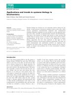
Figure 2: Classification map
The results were analyzed using clustering (Fig-
ure 2) and multidimensional scaling (Figure 3).
Clustering is a common technique in a statistical
data analysis based on a partition of a set of ob-
jects into groups or clusters (Manning and Schütze,
1999). Multidimensional scaling is data analysis
technique that provides a spatial display of the data
revealing relationships between the instances in the
data set (Davison, 1992). On both the maps the
biggest division is between East and West. The bor-
der between these two areas goes around Pleven and
Teteven, and it is the border of “yat” realization as
presented in the traditional dialectological atlases
(Stojkov, 2002). The most incoherent area is the
5
An interesting discussion on the normalization by length
can be found in Heeringa et al. (2006). In this paper the authors
report that contrary to results from previous work (Heeringa,
2004) non-normalized string distance measures are superior to
normalized ones.
63
area of Rodopi mountain, and the dialects present
in this area show the greatest similarity with the di-
alects found in the Southeastern part around Malko

Tyrnovo. On the map in Figure 3 it is also possible
to distinguish the area around Golica and Kozichino
on the East, which conforms to the maps found in
Stojkov (2002). Results of the aggregate analysis
conform both to the traditional maps presented in
Stojkov (2002), and to the work reported in Osen-
ova et al. (2007).
Figure 3: MDS map
4 Regular Sound Correspondences
The same data used for the aggregate analysis was
reused to extract sound correspondences and to iden-
tify underlying linguistic structure in the aggregate
analysis. The method and the obtained results will
be presented in more detail.
4.1 Method
From the aligned pairs of word pronunciations all
non-matching segments were extracted and sorted
according to their frequency. In the entire data set
there were 683 different pairs of sound correspon-
dences that appeared 955199 times.
e i 36565 j - 21361
@ È 26398 A @ 20515
o u 26108 e "e 19934
"6 "e 23689 r r
j
19787
v - 22100 "È - 18867
Table 1: Most frequent sound correspondences
The most frequent correspondences were taken to
be the most important sound alternations responsi-

ble for dialect variation. The method was tested on
the 10 most frequent correspondences which were
responsible for the 25% of sound alternations in the
whole data set.
In order to determine which of the extracted sound
correspondences is responsible for which of the di-
visions present in the aggregate analysis, each site
was compared to all other sites with respect to the
10 most frequent sound correspondences. For each
pair of sites all sound correspondences were ex-
tracted, including both matching and non-matching
segments. For further analysis it was important to
distinguish which sound comes from which place.
For each pair of the sound correspondences from
Table 1 a correspondence index is calculated for
each site using the following formula:
1
n
−
1
n

i=1,j=i
s
i
−→s

j
(1)
where n represents the number of sites, and s

i
−→s

j
the comparison of each two sites (i, j) with respect
to the sound correspondence s/s

. s
i
−→s

j
is calcu-
lated applying the following formula:
|s
i
, s

j
|
|s
i
, s

j
| + |s
i
, s
j
|

(2)
In the above formula s
i
and s

j
stand for the pair of
sounds involved in one of the most frequent sound
correspondences from Table1. |s
i
, s

j
|represents the
number of times s is seen in the word pronunciations
collected at site i, aligned with the s

in word pro-
nunciations collected at site j. |s
i
, s
j
| is the number
of times s stayed unchanged. For each pair of sound
correspondences a correspondence index was calcu-
lated for the s, s

correspondence, as well as for the
s


, s correspondence. For example, for the pair of
correspondences [e] and [i], the relation of [e] cor-
responding to [i] is separated from the relation of [i]
corresponding to [e].
6
For example, the indices for the sites Aldomirovci
and Borisovo with respect to the sound correspon-
dence [e]-[i] were calculated in the following way.
In the file with the sound correspondences extracted
from all aligned word pronunciations collected at
6
It would also be possible to modify this formula and calcu-
late the ratio of s to s corresponding to any other sound. In this
case the result would be a very small number of sites with the
very high correspondence index.
64
these two sites, the algorithm searches for pairs rep-
resented in Table 2:
Aldomirovci e i e
Borisovo i e e
no. of correspondences 24 0 3
Table 2: How often [e] corresponds to [i] and [e]
For each of the sites the indices were calculated us-
ing the above formula. The index for site i (Al-
domirovci) was:
|e, i|
|e, i| + |e, e|
=
24
24 + 3

= 0.89 (3)
The index for site j (Borisovo) was calculated in the
similar fashion from the Table 2:
|e, i|
|e, i| + |e, e|
=
0
0 + 3
= 0.00 (4)
Each of these two sites was compared to all other
sites with respect to the [e]-[i] correspondence re-
sulting in 83 indices for each site. The general cor-
respondence index for each site represents the mean
of all 83 indices. For the site i (Aldomirovci) gen-
eral index was 0.40, and for the site j (Borisovo)
0.21. Sites with the higher values of the general cor-
respondence index represent the sites where sound
[e] tends to be present, with respect to the [e]-[i]
correspondence (see Figure 4). In the same fash-
ion general correspondence indices were calculated
for every site with respect to each pair of the most
frequent correspondences (Table 1).
4.2 Results
The methods described in the previous section were
applied to all phone pairs from the Table 1, resulting
in 17 different divisions of the sites.
7
Data obtained by the analysis of sound correspon-
dences, i.e. indices of correspondences for sites was
used to draw maps in which every site is set off by

Voronoi tessellation from all other sites, and shaded
based on the value of the general correspondence in-
dex. Light polygons on the map represent areas with
7
For three pairs where one sound doesn’t have a correspond-
ing one (when there was an insertion or deletion) it is not pos-
sible to calculate an index. Formulas for comparing two sites
from the previous section would always give value 1 for the in-
dex.
the higher values of the correspondence index, i.e.
areas where the first sound in the examined alterna-
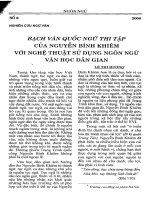
tion tends to be present. This technique enables us
to visualize the geographical distribution of the ex-
amined sounds. For example, map in Figure 4 rep-
Figure 4: Distribution of [e] sound
resents geographical distribution of sound [e] with
respect to the [e]-[i] correspondence, while map in
Figure 5 reveals the presence of the sound [i] with
respect to the [i]-[e] correspondence.
Figure 5: Distribution of [i] sound
In order to compare the dialect divisions obtained
by the aggregate analysis, and those based on the
general correspondence index for a certain phone
pair, correlation coefficient was calculated for these
2 sets of distances. The results are shown in Ta-
ble 3. Dialect divisions based on the [r]-[r
j
] and [i]-
[e] alternations have the highest correlation with the
distances obtained by the aggregate analysis. The

square of the Pearson correlation coefficient pre-
sented in column 3 enables us to see that 39.0% and
30.7% of the variance in the aggregate analysis can
be explained by these two sound alternations.
65
Correspondence Correlation r
2
x100(%)
[e]-[i] 0.19 3.7
[i]-[e] 0.55 30.7
[@]-[È] 0.26 6.7
[È]-[@] 0.23 5.3
[o]-[u] 0.49 24.4
[u]-[o] 0.43 18.9
["A]-["e] 0.49 24.3
["e]-["A] 0.38 14.2
[v]- - 0.14 2.0
[j]- - 0.20 4.0
[A]-[@] 0.51 26.5
[@]-[A] 0.26 7.0
[e]-["e] 0.18 3.2
["e]-[e] 0.23 5.2
[r]-[r
j
] 0.62 39.0
[r
j
]-[r] 0.53 28.1
["È]- - 0.17 2.9
Table 3: Correlation coefficient

5 Conclusion and Future Work
The dialect division of Bulgaria based on the aggre-
gate analysis presented in this paper conforms both
to traditional maps (Stojkov, 2002) and to the work
reported in Osenova et al. (2007), suggesting that
the novel data used in this project is representative.
The method of quantification of regular sound corre-
spondences described in the second part of the paper
was successful in the identification of the underlying
linguistic structure of the dialect divisions. It is an
important step towards more general investigation of
the role of the regular sound changes in the language
dialect variation. The main drawback of the method
is that it analyzes one sound alternation at the time,
while in the real data it is often the case that one
sound corresponds to several other sounds and that
sound correspondences involve series of segments.
In future work some kind of a feature represen-
tation of segments should be included in the anal-
ysis in order to deal with the drawbacks noted. It
would also be very important to analyze the context
in which examined sounds appear, since we can talk
about regular sound changes only with respect to the
certain phonological environments.
References
Mark L. Davison. 1992. Multidimensional scaling. Mel-
bourne, Fl. CA: Krieger Publishing Company.
Wilbert Heeringa, Peter Kleiweg, Charlotte Gooskens,
and John Nerbonne. 2006. Evaluation of String
Distance Algorithms for Dialectology. In John Ner-

bonne and Erhard Hinrichs, editors, Linguistic Dis-
tances. Workshop at the joint conference of Interna-
tional Committee on Computational Linguistics and
the Association for Computational Linguistics, Syd-
ney.
Wilbert Heeringa. 2004. Measuring Dialect Pronunci-
ation Differences using Levensthein Distance. PhD
Thesis, University of Groningen.
Grzegorz Kondrak. 2002. Algorithms for Language Re-
construction. PhD Thesis, University of Toronto.
Chris Manning and Hinrich Schütze. 1999. Founda-
tions of Statistical Natural Language Processing. MIT
Press. Cambridge, MA.
I. Dan Melamed. 2000. Models of translational equiv-
alence among words. Computational Linguistics,
26(2):221–249.
John Nerbonne. 2005. Various Variation Aggregates in
the LAMSAS South. In Catherine Davis and Michael
Picone, editors, Language Variety in the South III. Uni-
versity of Alabama Press, Tuscaloosa.
John Nerbonne. 2006. Identifying Linguistic Structure
in Aggregate Comparison. Literary and Linguistic
Computing, 21(4).
Petya Osenova, Wilbert Heeringa, and John Nerbonne.
2007. A Quantitive Analysis of Bulgarian Dialect
Pronunciation. Accepted to appear in Zeitschrift für
slavische Philologie.
Stojko Stojkov and Samuil B. Bernstein. 1964. Atlas of
Bulgarian Dialects: Southeastern Bulgaria. Publish-
ing House of Bulgarian Academy of Science, volume

I, Sofia, Bulgaria.
Stojko Stojkov, Kiril Mirchev, Ivan Kochev, and Mak-
sim Mladenov. 1974. Atlas of Bulgarian Dialects:
Southwestern Bulgaria. Publishing House of Bulgar-
ian Academy of Science, volume III, Sofia, Bulgaria.
Stojko Stojkov, Ivan Kochev, and Maksim Mladenov.
1981. Atlas of Bulgarian Dialects: Northwestern Bul-
garia. Publishing House of Bulgarian Academy of
Science, volume IV, Sofia, Bulgaria.
Stojko Stojkov. 1966. Atlas of Bulgarian Dialects:
Northeastern Bulgaria. Publishing House of Bulgar-
ian Academy of Science, volume II, Sofia, Bulgaria.
Stojko Stojkov. 2002. Bulgarska dialektologiya. Sofia,
4th ed.
66