Tài liệu Báo cáo khoa học: "An Evaluation Method of Words Tendency using Decision " docx

An Evaluation Method of Words Tendency using Decision Tree
El-Sayed Atlam, Masaki Oono, and Jun-ichi Aoe
Department of Information Science and Intelligent Systems
University of Tokushima
Tokushima,770-8506, Japan.
E-mail:


ABSTRACT
In every text, some words have frequency appearance
and are considered as keywords because they have
strong relationship with the subjects of their texts,
these words frequencies change with time-series
variation in a given period. However, in traditional
text dealing methods and text search techniques, the
importance of frequency change with time-series
variation is not considered. Therefore, traditional
methods could not correctly determine index of word’s
popularity in a given period. In this paper, a new
method is proposed to estimate automatically the
stability classes (increasing, relatively constant, and
decreasing) that indicate word’s popularity with time-
series variation based on the frequency change in past
texts data. At first, learning data was produced by
defining four attributes to measure frequency change
of word quantitatively, these four attributes were
extracted automatically from electronic texts.
According to the comparison between the
evaluation of the decision tree results and manually
(Human) results, F-measures of increasing, relatively

constant and decreasing classes were 0.847, 0.851,
and 0.768 respectively, and the effectiveness of this
method is achieved.

Keywords: time-series variation, words popularity,
decision tree, CNN newspaper
.

1. INTRODUCTION
Recently, there are many large electronic texts and
computers are processing (analysis) them widely.
Determination of important keywords is crucial in
successful modern Information Retrieval (IR). Usually,
frequency of some words in the texts are changing by
time (time-series variation), and these words are
commonly connected with particular period (e.g.
“influenza” is more common in winter). According to
Hisano (2000) some Chinese characters (Kanji) appear
in newspaper reports change with time-series
variation. Ohkubo et al. (1998) proposed a method to
estimate information that users might need in order to
analysis login data on a WWW search engine. By
Ohkubo method, it is confirmed that, word groups
connected with search words change according to time
when the search is done. Some words have a
frequency of use that changes with time-series
variation, and often those words attract the attention of
the users in a particular period. Such words are often
directly connected with the main subject of the text,
and can be considered as keywords that express

important characteristics of the text.
In traditional text dealing methods (Fukumoto,
Suzuki & Fukumoto, 1996; Hara, Nakajima & Kitani,
1997; Haruo, 1991; Sagara & Watanabe, 1998) and
text search techniques (Liman, 1996; Swerts &
Ostendorf, 1995), words frequency change with time-
series variation is not considered. Therefore, such
methods can not correctly determine the importance of
words in a given period (e.g. one-year). If the change
of word frequencies with time-series variation is
considered, especially when searching for similar
texts.
This paper presents a new method for
estimating automatically the stability classes that
indicate index of words popularity with time-series
variation based on frequency change in past texts data.
To estimate quantitatively the frequency change in the
time-series variation of words in each class, this
method defines four attributes (proper nouns
attributes, slope of regression line, slice of regression
line, and correlation coefficient) that are extracted
automatically from past texts data. These extracted
data are classified manually (Human) into three
stability classes. Decision Tree (DT) automatic
algorithm C4.5 (Quinlan, 1993; Weiss & Kulikowski,
1991; Honda, Mochizuki, Ho & Okumura, 1997;
Passonneau & Litman, 1997; Okumura, Haraguchi &
Mochizuki,1999) uses these data as learning data.
Finally, DT automatically determines the stability
classes of the input analysis data (test data).

2. POPULARITY OF WORDS
CONSIDERING TIME-SERIES
VARIATION
2.1 Stability Classes of the Words:
To judge the index of popularity of words with time-
series variation based on the frequency change, and
create the stability classes of the words, we defined
three classes as follow:
(1) Increasing Class “The class that has an increasing
frequency with time-series variation”
(2) Relatively Constant Class “The class that has a
stable frequency with time-series variation”
(3) Decreasing Class “The class that has a decreasing
frequency with time-series variation”.
We call these classes stability classes. The words
belong to each class is called:
increasing-words, relatively constant-words, and
decreasing-words respectively.
Table 1 shows a sample of some classified
words according to frequency change with time-series
variation in each stability class. For example, the
names of baseball players “Sammy-Sosa” and
“McGwire” are included in increasing class because
their frequencies increase with time-series variation.
The names of baseball teams “New-York-Mets” and
“Texas-Rangers” are included in a relatively constant
class because their frequencies relatively stable with
time-series variation. The names of baseball players
“Hank-Aaron” and “Nap Lajoie” are included in a

decreasing class because their frequencies decrease
with time-series variation.
Words stability classes are decided by the
change of their frequencies with time-series variation.
In order to determine the change of frequency with
time-series variation, texts were grouped according to
a given period (one-year) and frequency of words in
each group is estimated. However, to absorb the
influence caused by difference of number of texts in
each group and to judge the change with time-series
more correctly, each frequency is normalized by being
divided by the total frequencies of the words in each
group.
Table 1 Sample of Classified Words
Stability Class Example of words in each class
Increasing Words Sammy-Sosa, McGwire,
Carlos-Delgado

Relatively constant
words
Home-run, Coach, Baseball,
New-York-Mets, Texas-
Rangers
Decreasing words Hank-Aaron, Nolan-Ryan, Lou-
Gehrig, Babe-Ruth
In this paper, five attributes are defined to
decide the stability classes, and the words data that are
divided into classes beforehand are input into the DT
automatic algorithm C4.5 as the learning data. Then
we use the obtained DT to decide automatically the

stability classes of increasing words. In the next
section, the attributes that are used in the DT learning
to judge the stability classes will be described
.

3. ATTRIBUTES USED IN JUDGING
THE STABILITY CLASS
To obtain the characteristics of the change of word’s
frequencies quantitatively, the following attributes are
defined. The value of each attribute defined here is
used as the input data for the DT describe in section 4.
1) Proper Nouns Attributes (pna)
2) Slope of regression straight line (
α
)
3) Slice of regression straight line (
β
)
4) Correlation coefficient (r)

3.1 Proper Nouns Attributes (pna)
In this paper, we selected only three kinds of proper
nouns attributes: “Player-name”, “Organization-
name”, and “Team-name” to study the influence of the
time-series variation and to obtain the characteristics
of increasing or decreasing stability classes. Also we
used “Ordinary-nouns” (e.g. “ball”, “coach”, “home-
run”) for the relatively constant class. The
characteristics of the stability class are much easier
and more correct by using these entities analysis.

3.2 The Slope and the Slice of
Regression Straight Line (
α
&
β
):
Regression analysis is a statistical method, which
approximates the change of the sample value with
straight line in two dimension rectangular coordinates,
and this approximation straight line is called a
regression straight line (Gonick & Smith, 1993).
In this progress we take the standard years
(x
1
= first year, x
2
= second year,………x
i
= i year,
………, x
n
= n year) as a horizontal axis, and the
corresponding normalization frequency y
i
of the
words as a vertical axis. The slope segmentation
α
and
the slice

β
of the equation y =
α
x +
β
can be
calculated by the following formula:
)1(
)(
))((
1
2
1
ΛΛΛΛ
∑
∑
=
=
−
−−
=
n
i
i
n
i
ii
xx
yyxx
α

y
x
)2(ΛΛ
Λ
Λ
xy
α
β
−
=
where , are the average values of x
i
, y
i

respectively.
By obtaining the cross point of the regression
straight line and the current time period in rectangular
coordinates, it is possible to get the estimated
frequencies of the current words. The slope of the
regression straight line can estimate the stability
classes of the words. In addition, from the slice of the
regression straight line, the difference of frequencies
between words groups in the same stability class can
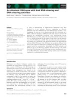
be estimated. For example the frequency of the words
in the same stability class (relatively constant) that
have a regression straight line (1) in Fig. 5 is higher
every period than that of straight line (2). The value of
the slice of regression straight line (1) is also higher
than that of regression straight line (2). So, we can

decide that the words of the regression straight line (1)
are more important than the words in the regression
straight line (2), even though all these words are in the
same class.
Freq.


●
●
○
○
○
●
○ ○
○ ○
●
●
●
(
1
)

4. ESTIMATION


In order to confirm the effectiveness of our method, an
experiment is designed to study the effect of learning
period lengths and all attributes on the distribution
precision of DT output, as explained below
:

(
2
)


Periods
)3(
)(
)
ˆ
(
)(
2
1
1
2
ΛΛΛΛΛ
yy
yy
ofsignr
n
i
i
n
i
i
−
−
=

∑
∑
=
=
α
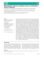
Fig. 1 Example of the difference of Important
Words group in a Similar Class.
By obtaining the cross point of the regression
straight line and the current time period in rectangular
coordinates, the slope of the regression straight line
can estimate the stability classes of the words. For
example, when the stability class is stabilized, the
regression straight line is close to the horizontal line
and the slope is close to 0. When the stability class is
increasing, its slope is positive, and the slope becomes
negative when the stability class is decreasing.


In addition, from the slice of the regression
straight line, the difference of frequencies between
words groups in the same stability class can be
estimated. For example the frequency of the words in
the same stability class (relatively constant) that have a
regression straight line (1) in Fig. 1 is higher every
period than that of straight line (2). The value of the
slice of regression straight line (1) is also higher than
that of regression straight line (2). So, we can decide
that the words of the regression straight line (1) are
more important than the words in the regression
straight line (2), even though all these words are in the

same class.

3.3. Correlation Coefficient (r)
Correlation coefficient is used to judge the reliability
of regression straight line. Although, stability classes
of words are estimated by slope and slice of the
regression straight line, there are some words with the
same regression straight line have versus degree of
scattering because of the arrangement of frequencies
of words in rectangular coordinates as shown in Fig. 2.
In such case, there will be some problems in the point
of reliability if these different groups of words have
the same stability class.
So, in order to judge the reliability of the regression
straight line that derived from the scattering of
frequencies, a correlation coefficient was used that
shows the scattering extent (degree) of the frequencies
of words in rectangular coordinates. Correlation
coefficient is also a statistical method (Gonick &
Smith, 1993), and the calculation equation is shown as
follows: In the above formula,
are the predicted
weights determined by regression line and
α
is the
slope of the regression straight line.
i
y
ˆ
When the absolute value of correlation

coefficient r is approaching to 1, the appearance
frequency is concentrated around the regression
straight line, and when it approaches to 0, it means that
the appearance frequency is irregularly scattering
around the regression straight line.



Ferq.


Periods
Fig. 2 An Illustration of Regression
Coefficient.

4.1 Experimental Data:
The sports section of CNN newspapers (1997-2000)
was used as an experimental collection data, because
of the uniqueness of the words in this field
and their tendency to change with the time-series
variation. A specific sub-field from sports
“professional baseball” was chosen because it has
stabilized frequent reports every year, and it is
relatively easy to determine how words frequencies
affect by time-series variation. Words identify with
four kinds of proper nouns attributes: “Player-name”,
“Organization-name”, “Team-name”, and “Ordinary-
nouns” were extracted from the selected reports, and
the normalized frequency of the selected words in each
year was obtained. Then, stability classes classified

manually (Human) to these words.
The data is divided into two groups: one
includes the reports of years (1997- 1999) are used
as DT learning data. The other includes the reports of
years (1997-2000), that are completely different data
than the learning data, are used as test data. For both
data sets the attributes are obtained from the change of
words frequency with time- series variation included
in both periods. The data of extracted words is shown
in Table 2.
In order to get the accuracy of the correct words that
are words that are evaluated automatically by DT
, we measured: Precision (P), and Recall (R) rate as
follows:
Number of correct words extracted by (DT)
Precision =
Total number of words extracted by (DT)

Number of correct words extracted by DT)
Recall =
❈
❈
❈
❈
❈
❈
Total number of correct words classified manually
Table 2 Evaluation Data.
DT Learning Data DT Test Data
M N X Y

Period
1997-1999 1998-1999 1997-2000 1998-2000
Total Number of Words
443 360 472 392
Increasing Words
55 59 69 82
Constant Words
243 187 252 200
Decreasing Words
145 114 151 110

Table 3 Relation between various periods of time and Classification Precision.
Learning Period
N (1998-1999) M (1997-1999)
Classes
I C D I C D
Precision
49.41 73.48 65.9 82.73 97.13 65.68
Recall
63.36 49.77 95 84.73 75.78 92.5
Where “i, c, d” are increasing, relatively constant and decreasing classes
4.2 Relation Between Learning Period
and Classification Precision:
In this section, we show the effectiveness of using
the longest period M and the shortest period N of
learning data to distribution of P & R. We notice
that, when the period of learning data is longer (M)
the number of words increases and characteristics
of the relatively constant and decreasing stability
classes become more obvious, so their

classifications become clear, and as a result P & R
become higher. However, when short learning
period is used P & R decrease. The comparison
results for the longest and shortest periods are
shown in Table 3.

5. CONCLUSION
Stability classes are defined as the index of popularity
of words, and five attributes are defined to obtain the
frequency change of words quantitatively. The method
is proposed to estimate automatically stability classes of
words by having DT learning to be done on extracted
attributes from past text data. It is confirmed by the test
results that classification precision can be improved
when all five attributes and the longest learning period
are used
. Future work could focus on texts in fields
other than sports that is used in this paper

REFERENCES
Fukumoto, F., Suzuki, Y., & Fukumoto, J.I.
(1996). An Automatic Clustering of Articles Using
Dictionary Definitions. Trans. Of Information
Processing Society of Japan, 37(10), (pp. 1789-
1799).
Gonick, L., & Smith, W. (1993). The Cartoon
Guide to Statistics, HarperCollins Publishers.
Hara, M., Nakajima, H., & Kitani, T. (1997).
Keyword Extraction Using Text Format and Word
Importance in Specific Field. Trans. Of

Information Processing Society of Japan, 38(2),
(pp. 299-309).
Haruo, K. (1991). Automatic Indexing and
Evaluation of Keywords for Japanese Newspaper.
Trans. of the Institute of Electronics, Information
and Communication Engineering (IEICE). J74-D-I
(8), (pp. 556-566).
Hisano, H. (2000). Page-Type and Time-Series
Variations of a Newspaper's Character Occurrence
Rate., Journal of Natural Language Processing, 7
(2), (pp.45-61).
Honda, T., Mochizuki, H., Ho,T.B., & Okumura,
M. (1997). Generating Decision Trees from an
Unbalanced Data Set. In proceeding of the 9
th

European Conference on Machine Learning.
Liman, J. (1996). Cue Phrase Classification Using
Machine Learning. Journal of Artificial
Intelligence Research, 5, (pp. 53-94).
Okumura, M., Haraguchi, Y., & Mochizuki, H.
(1999). Some Observation on Automatic Text
Summarization Based on Decision Tree Learning.
Journal of Information Processing Society of
Japan. No.5N-2,(pp. 71-72).
Ohkubo, M., Sugizaki, M., Inoue, T., & Tanaka,
K. (1998). Extracting Information Demand by
Analyzing a WWW Search Login. Trans. of
Information Processing Society of Japan, 39(7),
(pp. 2250-2258).

Passonneau, R.J., & Litman, D.J. (1997).
Discourse Segmentation by Human and
Automated Means. Computational Linguistics, 23
(1), (pp. 103-139).
Quinlan, J.R. (1993). C4.5: Programs for
Machine Learning , Morgan Kaufmann.
Sagara, K., & Watanabe, K. (1998). Extraction of
Important Terms that Reflect the Contents of
English Contracts. Journal of Special Interest
Groups of Natural
Language & Information Processing Society of
Japan (SIGNL-IPSJ), (pp. 91-98).
Salton, G., & McGill, M.J. (1983). Introduction of
Modern Information Retrieval. New York
McGraw-Hill