Tài liệu Báo cáo khoa học: "Prefix Probabilities from Stochastic Tree Adjoining Grammars*" pptx

Prefix Probabilities from Stochastic Tree Adjoining Grammars*
Mark-Jan Nederhof
DFKI
Stuhlsatzenhausweg 3,
D-66123 Saarbriicken,
Germany
nederhof@dfki, de
Anoop Sarkar
Dept. of Computer and Info. Sc.
Univ of Pennsylvania
200 South 33rd Street,
Philadelphia, PA 19104 USA
anoop©linc, cis. upenn, edu
Giorgio Satta
Dip. di Elettr. e Inf.
Univ. di Padova
via Gradenigo 6/A,
35131 Padova, Italy
satta@dei, unipd, it
Abstract
Language models for speech recognition typ-
ically use a probability model of the form
Pr(an[al,a2, ,an-i).
Stochastic grammars,
on the other hand, are typically used to as-
sign structure to utterances, A language model
of the above form is constructed from such
grammars by computing the prefix probabil-
ity ~we~* Pr(al artw), where w represents
all possible terminations of the prefix
al an.

The main result in this paper is an algorithm
to compute such prefix probabilities given a
stochastic Tree Adjoining Grammar (TAG).
The algorithm achieves the required computa-
tion in O(n 6) time. The probability of sub-
derivations that do not derive any words in the
prefix, but contribute structurally to its deriva-
tion, are precomputed to achieve termination.
This algorithm enables existing corpus-based es-
timation techniques for stochastic TAGs to be
used for language modelling.
1 Introduction
Given some word sequence
al'.'an-1,
speech
recognition language models are used to hy-
pothesize the next word
an,
which could be
any word from the vocabulary F~. This
is typically done using a probability model
Pr(an[al, ,an-1).
Based on the assumption
that modelling the hidden structure of nat-
* Part of this research was done while the first and the
third authors were visiting the Institute for Research
in Cognitive Science, University of Pennsylvania. The
first author was supported by the German Federal Min-
istry of Education, Science, Research and Technology
(BMBF) in the framework of the VERBMOBIL Project un-

der Grant 01 IV 701 V0, and by the Priority Programme
Language and Speech Technology, which is sponsored by
NWO (Dutch Organization for Scientific Research). The
second and third authors were partially supported by
NSF grant SBR8920230 and ARO grant DAAH0404-94-
G-0426. The authors wish to thank Aravind Joshi for
his support in this research.
ural language would improve performance of
such language models, some researchers tried to
use stochastic context-free grammars (CFGs) to
produce language models (Wright and Wrigley,
1989; Jelinek and Lafferty, 1991; Stolcke, 1995).
The probability model used for a stochas-
tic grammar was ~we~* Pr(al anw). How-
ever, language models that are based on tri-
gram probability models out-perform stochastic
CFGs. The common wisdom about this failure
of CFGs is that trigram models are lexicalized
models while CFGs are not.
Tree Adjoining Grammars (TAGs) are impor-
tant in this respect since they are easily lexical-
ized while capturing the constituent structure
of language. More importantly, TAGs allow
greater linguistic expressiveness. The trees as-
sociated with words can be used to encode argu-
ment and adjunct relations in various syntactic
environments. This paper assumes some famil-
iarity with the TAG formalism. (Joshi, 1988)
and (Joshi and Schabes, 1992) are good intro-
ductions to the formalism and its linguistic rele-

vance. TAGs have been shown to have relations
with both phrase-structure grammars and de-
pendency grammars (Rambow and Joshi, 1995),
which is relevant because recent work on
struc-
tured
language models (Chelba et al., 1997) have
used dependency grammars to exploit their lex-
icalization. We use stochastic TAGs as such a
structured
language model in contrast with ear-
lier work where TAGs have been exploited in
a class-based n-gram language model (Srinivas,
1996).
This paper derives an algorithm to compute
prefix probabilities ~we~* Pr(al
anw).
The
algorithm assumes as input a stochastic TAG G
and a string which is a prefix of some string in
L(G),
the language generated by G. This algo-
rithm enables existing corpus-based estimation
techniques (Schabes, 1992) in stochastic TAGs
to be used for language modelling.
953
2 Notation
A stochastic Tree Adjoining Grammar (STAG)
is represented by a tuple
(NT,

E,:T, .A, ¢) where
NT
is a set of nonterminal symbols, E is a set
of terminal symbols, 2: is a set of
initial
trees
and .A is a set of auxiliary trees. Trees in :TU.A
are also called elementary trees.
We refer to the root of an elementary tree t as
Rt.
Each auxiliary tree has exactly one distin-
guished leaf, which is called the foot. We refer
to the foot of an auxiliary tree t as Ft. We let
V denote the set of all nodes in the elementary
trees.
For each leaf N in an elementary tree, except
when it is a foot, we define
label(N)
to be the
label of the node, which is either a terminal from
E or the empty string e. For each other node
N, label(N)
is an element from
NT.
At a node N in a tree such that
label(N) •
NT
an operation called adjunction can be ap-
plied, which excises the tree at N and inserts
an auxiliary tree.

Function ¢ assigns a probability to each ad-
junction. The probability of adjunction of t • A
at node N is denoted by ¢(t, N). The probabil-
ity that at N no adjunction is applied is denoted
by ¢(nil, N). We assume that each STAG G
that we consider is proper. That is, for each
N such that
label(N) • NT,
¢(t, N) = 1.
tE.AU{nil}
For each non-leaAf node N we construct the
string
cdn(N) = N1 Nm
from the (ordered)
list of children nodes
N1, ,Nm
by defining,
for each d such that 1 < d < m,
Nd = label(Nd)
in case
label(Nd)
• E U {e}, and
N d
=
Nd
oth-
erwise. In other words, children nodes are re-
placed by their labels unless the labels are non-
terminal symbols.
To simplify the exposition, we assume an ad-

ditional node for each auxiliary tree t, which
we denote by 3_. This is the unique child of the
actual foot node Ft. That is, we change the def-
inition of
cdn
such that
cdn(Ft) = 2_
for each
auxiliary tree t. We set
V ± = {N e V I label(N) • NT} U E U {3_}.
We use symbols a,b,c, , to range over E,
symbols
v,w,x, ,
to range over E*, sym-
bols N, M, to range over V ±, and symbols
~, fl, 7, to range over (V±) *. We use t, t',
to denote trees in 2: U ,4 or subtrees thereof.
We define the predicate
dft
on elements from
V ± as dft(N)
if and only if (i) N E V and N
dominates 3_, or (ii) N = 3_. We extend dft
to strings of the form N1 Nm
E (V±) *
by
defining
dft(N1 Nm)
if and only if there is a
d (1 < d < m) such that

dft(Nd).
For some logical expression p, we define
5(p) = 1 iff p is true, 5(p) = 0 otherwise.
3 Overview
The approach we adopt in the next section to
derive a method for the computation of prefix
probabilities for TAGs is based on transforma-
tions of equations. Here we informally discuss
the general ideas underlying equation transfor-
mations.
Let
w = ala2 an E ~*
be a string and let
N E V ±. We use the following representation
which is standard in tabular methods for TAG
parsing. An item is a tuple [N,
i, j, fl,
f2] rep-
resenting the set of all trees t such that (i) t is a
subtree rooted at N of some derived elementary
tree; and (ii) t's root spans from position i to
position j in w, t's foot node spans from posi-
tion fl to position
f2
in w. In case N does not
dominate the foot, we set fl = f2 = We gen-
eralize in the obvious way to items It, i, j, fl, f2],
where t is an elementary tree, and [a, i, j, fl, f2],
where
cdn (N) = al~

for some N and/3.
To introduce our approach, let us start with
some considerations concerning the TAG pars-
ing problem. When parsing w with a TAG G,
one usually composes items in order to con-
struct new items spanning a larger portion of
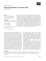
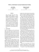
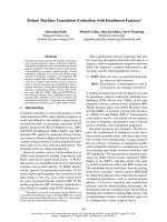
the input string. Assume there are instances of
auxiliary trees t and t' in G, where the yield of
t', apart from its foot, is the empty string. If
¢(t, N) > 0 for some node N on the spine of t',
and we have recognized an item
[Rt, i,j, fl, f2],
then we may adjoin t at N and hence deduce
the existence of an item
[Rt,,i,j, fl, f2]
(see
Fig. l(a)). Similarly, if t can be adjoined at
a node N to the left of the spine of t' and
fl = f2, we may deduce the existence of an item
[Rt, , i, j, j, j]
(see Fig. l(b)). Importantly, one
or more other auxiliary trees with empty yield
could wrap the tree t' before t adjoins. Adjunc-
tions in this situation are potentially nontermi-
hating.
One may argue that situations where auxil-
iary trees have empty yield do not occur in prac-
tice, and are even by definition excluded in the
954
(a) R t,

t t ~
(b) R,,
Figure 1: Wrapping in auxiliary trees with
empty yield
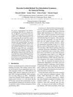
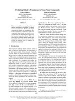
case of lexicalized TAGs. However, in the com-
putation of the prefix probability we must take
into account trees with non-empty yield which
behave like trees with empty yield because their
lexical nodes fall to the right of the right bound-
ary of the prefix string. For example, the two
cases previously considered in Fig. 1 now gen-
eralize to those in Fig. 2.
Rt* Rtl
e~spine
i f~f2 n i
flff/~2 n
E
C
Figure 2: Wrapping of auxiliary trees when
computing the prefix probability
To derive a method for the computation of
prefix probabilities, we give some simple recur-
sive equations. Each equation
decomposes
an
item into other items in all possible ways, in
the sense that it expresses the probability of
that item as a function of the probabilities of
items associated with equal or smaller portions
of the input.

In specifying the equations, we exploit tech-
niques used in the parsing of incomplete in-
put (Lang, 1988). This allows us to compute
the prefix probability as a by-product of com-
puting the inside probability.
In order to avoid the problem of nontermi-
nation outlined above, we transform our equa-
tions to remove infinite recursion, while preserv-
ing the correctness of the probability computa-
tion. The transformation of the equations is
explained as follows. For an item I, the span
of I, written
a(I),
is the 4-tuple representing
the 4 input positions in I. We will define an
equivalence relation on spans that relates to the
portion of the input that is covered. The trans-
formations that we apply to our equations pro-
duce two new sets of equations. The first set
of equations are concerned with all possible de-
compositions of a given item I into set of items
of which one has a span equivalent to that of I
and the others have an empty span. Equations
in this set represent endless recursion. The sys-
tem of all such equations can be solved indepen-
dently of the actual input w. This is done once
for a given grammar.
The second set of equations have the property
that, when evaluated, recursion always termi-
nates. The evaluation of these equations com-

putes the probability of the input string modulo
the computation of some parts of the derivation
that do not contribute to the input itself. Com-
bination of the second set of equations with the
solutions obtained from the first set allows the
effective computation of the prefix probability.
4 Computing
Prefix Probabilities
This section develops an algorithm for the com-
putation of prefix probabilities for stochastic
TAGs.
4.1 General equations
The prefix probability is given by:
Pr(al anw)
= ~ P([t,O,n,-,-]),
wEE* fEZ
where P is a function over items recursively de-
fined as follows:
P([t,i,j, fl,f2]) = P([Rt, i,j, fl,f2]);
(1)
P([t~N,i,j,-,-])
= (2)
P([a,i,k,-,-]) . P([N,k,j,-,-]),
k(i < k < j)
if a ¢ e A -~dft(aN);
P([t~N, i, j, fl,
f2]) = (3)
Z P([a,i,k,-,-])-P([N,k,j, fl,f2]),
k(i < k < fl)
if ~ ¢ ¢ A dft(g);

955
P([aN, i, j, fl,
f2]) = (4)
P([a, i, k, fl,
f2]).
P([N, k, j, -,
-]),
k(f2 <_ k <_ j)
if # c ^
P([N, i, j, fl,/2])
= (5)
¢(nil,
N). P([cdn(N), i,j, fl,
f2]) +
P([cdn(N), f~, f~, f~, f2]) .
f~,f~(i S f~ S fl A f2 ~_ flo S J)
¢(t,
N). P([t, i,j, f[,
f~]),
tEA
if N • V A dft(N);
P([g,i,j,-,-])
= (6)
¢(nil,
N) . P([cdn(N), i,j,-,-])
+
P([cdn(N), f~, f~, -, -]) .
y~ ¢(t, N).
P([t,i,j,f[,f~]),
tEA

if N • V A
-,dfl(N);
P([a,i,j,-,-])
= (7)
+ 1 = j ^ aj = a) + = j = n);
P([-l-,i,j, fl,f2])
= (f(i = fl Aj = f2); (8)
P([e, i,j, -,
-]) = (f(i = j). (9)
Term
P([t, i, j, fl,
f2]) gives the inside probabil-
ity of all possible trees derived from elementary
tree t, having the indicated span over the input.
This is decomposed into the contribution of each
single node of t in equations (1) through (6).
In equations (5) and (6) the contribution of a
node N is determined by the combination of
the inside probabilities of N's children and by
all possible adjunetions at N. In (7) we rec-
ognize some terminal symbol if it occurs in the
prefix, or ignore its contribution to the span if it
occurs after the last symbol of the prefix. Cru-
cially, this step allows us to reduce the compu-
tation of prefix probabilities to the computation
of inside probabilities.
4.2 Terminating equations
In general, the recursive equations (1) to (9)
are not directly computable. This is because
the value of

P([A, i, j, f,
if]) might indirectly de-
pend on itself, giving rise to nontermination.
We therefore rewrite the equations.
We define an equivalence relation over spans,
that expresses when two items are associated
with equivalent portions of the input:
(i',j', f~, f~) .~ (i,j, fl,
f2) if and only if
((i',j') = (i,j))A
= (fl, f2)v
((f~ = f~ = iV f{ = f~ = jV f{
= f~ = )A
(fl = :2 = ivfl = f2 = jvf = :2 = -)))
We introduce two new functions P~ow and
P, pm. When evaluated on some item I, Plow re-
cursively calls itself as long as some other item
I'
with a given elementary tree as its first com-
ponent can be reached, such that a(I) ~.
a(I').
Pto~ returns 0 if the actual branch of recursion
cannot eventually reach such an item I', thus
removing the contribution to the prefix proba-
bility of that branch. If item I ' is reached, then
P~ow switches to
Psptit.
Complementary to Plow,
function
P, pm

tries to decompose an argument
item I into items I ~ such that
a(I) ~ a(I').
If
this is not possible through the actual branch
of recursion, P, pm returns 0. If decomposition
is indeed possible, then we start again with Pto,o
at items produced by the decomposition. The
effect of this intermixing of function calls is the
simulation of the original function P, with Pzo~
being called only on potentially nonterminating
parts of the computation, and P, pm being called
on parts that are guaranteed to terminate.
Consider some derivation tree spanning some
portion of the input string, and the associated
derivation tree 7 There must be a unique ele-
mentary tree which is represented by a node in
7- that is the "lowest" one that entirely spans
the portion of the input of interest. (This node
might be the root of T itself.) Then, for each
t E .A and for each
i,j, fl,f2
such that i < j
and i < fl < f2 __< j, we must have:
P([t, i, j,
fl, f2]) = (10)
l l • . I l
t' E
.A, fl,f~((z,3, fl,f~)
,~

(i,j, f1,f2))
Similarly, for each t E 27 and for each i, j such
that i < j, we must have:
P([t,i,j,
-, -1) = (11)
[t', L/]).
t' e {t} u.4,/~
{-,i,j}
The reason why P~o~, keeps a record of indices
f{ and
f~,
i.e., the spanning of the foot node
of the lowest tree (in the above sense) on which
Plow is called, will become clear later, when we
introduce equations (29) and (30).
We define
Pzo~:([t,i,j, fl,f2],[t',f[,f~])
and
P~o=([a,i,j, fl,f2],[t',f{,f~])
for / < j and
• . ! !
(i,j, fl,f2) ~ (z,3, fl,f~) ,
as follows.
956
Pto~o([t, i, j, fl, f2], [tt, f{,f~]) = (12)
Pto~o([Rt, i, j, fl,
f2],
[tt, f{,f~]) +
6((t,
fl, f2)

= (it,
fl, f2)) "
P,,m([nt, i, j,
fl,
f2]);
Pzo~([aN, i,j, -, -1, [t, f{,
f~]) = (13)
j,-,-],
P([N,j,j,-,-]) +
P([a,
i, i, -,
-])
•
P~o~.([N,i,j,-,-],
[t, f~, f~]),
if
a # e A ",dfl(aN);
P~o~([ag, i,j, ft,f2], [t,f{,f~])
= (14)
6(fl j)" Pto~([a, i,j,-, -], [t, f{, foil) •
P([N,j,j,
fl, f2])
+
P([a, i, i, -,
-]) •
Pto~,([g,i,j, fl,f2],
[t,f~,f~]),
if a # e A rift(N);
P,o~([aN, i,j, fx,f2], [t,f{,f~])
= (15)

P~o~([a,i,j,f~,f2],
[t, f~, f~]) •
P([N,j,j,-,-])
+
6(i = f2)" P([a, i, i, fl, f2]) "
P~o~([N,i,j,-,-], [t,f~,f~]),
if a # e A dft(a);
P~o~,([N, i, j, fl,
f2], [t, f{, f~]) : (16)
¢(nil, N) •
Pzo~ ([cdn
(N), i, j, fl, f2], [t, f{, f~]) +
P~o,o([cdn(N), i,j, fl,
f2], [t, fl, f~]) •
Et'eA
¢(t',
g) . P([t', i,j, i,j]) +
P([cdn(N),
fl,
f2, fl, f2]) "
E ¢(t', N). Pto~ ([t',
i,j,
fl, f21, [t, f{,
f~]),
t I E .4
if N E V A dft (N);
Pto~ ([N, i, j, -, -], [t, fl, f~]) = (17)
¢(nil, N) •
Pzo~,([cdn(N),i,j,-,-], [t,f{,f~]) +
P~o~([cdn(N), i,j,

-,-], [t, f{, f~]) •
Et'eA ¢(t',
N) . P([t', i, j, i,
j]) +
P([ cdn( g), f{', f~, -, -]) "
fl',f~'(fl'
= S~' = ~vy~' = S~' =~)
E ¢(t',
N)"P~ow ([t', i, j,
ill',
f2'], [t,
f{,
f~]),
t'EA
if N E V A -~dft(N);
Pto~([a,
i,j,
-, -], [t, f{, f~]) = O; (18)
Pto~,([-L,i,j, fl,f2], [t,f{,f¢.]) =
0; (19)
i,j, -, -], [t, = 0. (20)
The definition of Pto~ parallels the one of P
given in §4.1. In (12), the second term in the
right-hand side accounts for the case in which
the tree we are visiting is the "lowest" one on
which Pto,. should be called. Note how in the
above equations Pto~ must be called also on
nodes that do not dominate the footnode of the
elementary tree they belong to (cf. the definition
of ~). Since no call to P,p,t is possible through

the terms in (18), (19) and (20), we must set
the right-hand side of these equations to 0.
The specification of
P.pm([a, i, j, fl,f2])
is
given below. Again, the definition parallels the
one of P given in §4.1.
P, pm([aN, i, j, -,
-]) = (21)
P([a,i,k,-,-]) . P([Y,k,j,-,-]) +
k(i < k < j)
P, pm([a,i,j,-,-]) . P([Y,j,j,-,-])
+
P([a,i,i,-,-]) . P,p,,t([Y,i,j,-,-]),
if a # e A
-,dft(aN);
P, pm([aY, i, j, f l ,
f2]) =
(22)
E P([a,i,k,-,-]).P([N,k,j, fl,f2]) +
k(i<k< flAk<3)
~(fl
=
J) " P.p,t([a, i,j,-,-])
•
P([g,j,j, fl,f2]) +
P([a, i, i, -, -]).
P,,m([N, i, j,
fl, f2]),
if a # e A

dft(N);
Pspt,t
([aN, i, j, fl,
f2]) =
(23)
E P([a,i,k, fl,f2])" P([N,k,j,-,-])
+
k(i <kA f2 <k <j)
P.pm([a, i,j,
fl, f2])"
P([N,j,j, -,
-]) +
5(i = f2)" P([ot, i, i, fl, f2])"
P,,m([N,i,j,-,-1),
if a # e A
dfl(a);
Pop,,t([N, i, j, fl,
f2]) = (24)
¢(nil,
g). P~pm([cdn(N), i,j, fl,
f2]) +
y~ P([cdn(N),f~,f~,fl, f2]) "
fl,f~ (i < fl < f~ ^ f2 < f; < j ^
(fl,f~) •
(i,3) ^ (fl, f2) ¢
(fl,f2))
¢(t,
N) . P([t, i, j, f~,
f~]) +
tEA

P ,i,
([cdn
(N), i, j, fl,
f2]) •
¢(t,
g) . P([t, i, j, i,
j]),
tfA
957
if N E V A dft(N);
P,,,, ([N, i, j, -, -]) = (25)
¢(nil,
N). Psplit ([cdn (N), i, j, -,
-]) +
P([cdn(N), f~, f~, -, -]) .
l I ! I
*A
l I
fl'f2 (i< fl <_f~ < 3 (f~,f~)~(i,j)A
"~(fl -~f2 =ivfl = f2 =J))
¢(t,N).
P([t,i,j,f~,f~]) +
tEA
Ps,u, ([cdn ( N), i, j, -,
-])
¢(t,Y).
P([t,i,j,i,j]),
tEA
if N E Y A rift(N);
P.put([a,i,j, , ])

(~(i -t- 1 = j A
aj
= a); (26)
P, pm
([_1_, i, j, fl, f2]) = 0; (27)
P,,,,,([e, i,j, -,
-]) = 0. (28)
We can now separate those branches of re-
cursion that terminate on the given input from
the cases of endless recursion. We assume be-
low that
P,p,,([Rt, i,j,
f~,f~]) > 0. Even if this
is not always valid, for the purpose of deriving
the equations below, this assumption does not
lead to invalid results. We define a new function
Po, ,
which accounts for probabilities of sub-
derivations that do not derive any words in the
prefix, but contribute structurally to its deriva-
tion:
Po,t~.([t,i,j, fl,f2], [t',f~,f~_])
= (29)
Pto=([t,i,j, fz,f2], [t',f~,f~]).
I
" *
I I
P,,,i,
([Rt, *, 3,

fl, f~])
Po~t,,([a,i,j, Yl,:2], [t',:~,:~])
= (30)
P~o= ([a,
i,j,
fl, f2], [t', f~, f~])
P,,m
(iRe, i, j, f{, fgt])
We can now eliminate the infinite recur-
sion that arises in (10) and (11) by rewriting
P([t, i, j, fl, f2]) in terms of
Po.,,,:
P([t, i,j,
fy,/2]) = (31)
Po.,e,([t,i,j, fz,f2],
[t',f~,f~]).
l I
i
" I
tte A, fl,f2(( 'J'fl'f2) ~" (i,j, fl,f2))
P,,m([nt, , i,j, f~,
f~]);
P([t, i, j, -,
-]) = (32)
Po,t,~([t,i,j,-,-], [t',f,f]).
t' e
{t}
U.A,f E { ,i,j}
P, pzit
([Rt,, i, j, f, f]).

Equations for
Po~,,
will be derived in the next
subsection.
In summary, terminating computation of pre-
fix probabilities should be based on equa-
tions (31) and (32), which replace (1), along
with equations (2) to (9) and all the equations
for P, pm.
4.3 Off-line Equations
In this section we derive equations for function
Po~t,r
introduced in §4.2 and deal with all re-
maining cases of equations that cause infinite
recursion.
In some cases, function P can be computed
independently of the actual input. For any
i < n we can consistently define the following
quantities, where t E Z U.4 and a E V ± or
cdn(N) = aft
for some N and fl:
Ht = P([t,i,i,f,f]);
Ha = P([c~,i,i,f',f']),
where f = i if t E .A, f = - otherwise, and ff =
i if dft(a), f = - otherwise. Thus, Ht is the
probability of all derived trees obtained from t,
with no lexical node at their yields. Quantities
Ht and Ha can be computed by means of a sys-
tem of equations which can be directly obtained
from equations (1) to (9). Similar quantities as

above must be introduced for the case i = n.
For instance, we can set
H~ = P([t, n, n, f,
f]),
f specified as above, which gives the probabil-
ity of all derived trees obtained from t (with no
restriction at their yields).
Function
Po~e.
is also independent of the
actual input. Let us focus here on the case
fl,f2 ¢; {i,j,-}
(this enforces (fl, f2) = (f~, f~)
below). For any i, j, fl, f2 < n, we can consis-
tently define the following quantities.
Lt,t, = Po~te,([t,i,j, fl,f2], [t',f~,f~]);
L~,t, = Po.,°.([a,i,j, fl,f2], [t',f~,f~]).
In the case at hand,
Lt,t,
is the probability of all
derived trees obtained from t such that (i) no
lexical node is found at their yields; and (ii) at
some 'unfinished' node dominating the foot of
t, the probability of the adjunction of t ~ has al-
ready been accounted for, but t t itself has not
been adjoined.
It is straightforward to establish a system of
equations for the computation of
Lt,t,
and

La,t,,
by rewriting equations (12) to (20) according
to (29) and (30). For instance, combining (12)
and (29) gives (using the above assumptions on
fl
and
f2):
Lt,t' = LRt,t' + (~(t = t').
Also, if a ~ e and dft(N), combining (14)
and (30) gives (again, using previous assump-
958
tions on fl and f2; note that the
Ha's
are known
terms here):
L~N,t' =
Ha"
LN,t'.
For any i, fl,f2 <
n
and j = n, we also need to
define:
L~,t, = Po,,,.([t,i,n, fl,f2], [t',f~,f~]);
L:.t, = Po~, ([a,i,n, fx,f2],
[t',/~,/.~]).
Here
L~, t,
is the probability of all derived trees
obtained from t with a node dominating the
foot node of t, that is an adjunction site for t'

and is 'unfinished' in the same sense as above,
and with lexical nodes only in the portion of
the tree to the right of that node. When we
drop our assumption on fl and f2, we must
(pre)compute in addition terms of the form
Po~t~r([t,i,j,i,i],
[t',i,i]) and
Po~,~([t,i,j,i,i],
[t',j,j]) for i
<
j
<
n, Po,t~,([t,i,n, fl,n],
[t',/i,f~]) for
i < 11 < n,
Po,, ([t,i,n,n,n],
[t', f{, f~]) for i < n, and similar. Again, these
are independent of the choice of i, j and fl. Full
treatment is omitted due to length restrictions.
5 Complexity and concluding
remarks
We have presented a method for the computa-
tion of the prefix probability when the underly-
ing model is a Tree Adjoining Grammar. Func-
tion P,p,t is the core of the method. Its equa-
tions can be directly translated into an effective
algorithm, using standard functional memoiza-
tion or other tabular techniques. It is easy to
see that such an algorithm can be made to run
in

time O(n6),
where n is the length of the input
prefix.
All the quantities introduced in §4.3
(Ht,
Lt,t,,
etc.) are independent of the input and
should be computed off-line, using the system of
equations that can be derived as indicated. For
quantities
Ht
we have a non-linear system, since
equations (2) to (6) contain quadratic terms.
Solutions can then be approximated to any de-
gree of precision using standard iterative meth-
ods, as for instance those exploited in (Stolcke,
1995). Under the hypothesis that the grammar
is consistent, that is Pr(L(G)) = 1, all quanti-
ties H~ and H~ evaluate to one. For quantities
Lt,t,
and the like, §4.3 provides linear systems
whose solutions can easily be obtained using
standard methods. Note also that quantities
La,t,
are only used in the off-line computation
of quantities
Lt,t,,
they do not need to be stored
for the computation of prefix probabilities (com-
pare equations for

Lt,t,
with (31) and (32)).
We can easily develop implementations of our
method that can compute prefix probabilities
incrementally. That is, after we have computed
the prefix probability for a prefix al
an,
on in-
put an+l we can extend the calculation to prefix
al""anan+l
without having to recompute all
intermediate steps that do not depend on
an+l.
This step takes time O(n5).
In this paper we have assumed that the pa-
rameters of the stochastic TAG have been pre-
viously estimated. In practice, smoothing to
avoid sparse data problems plays an important
role. Smoothing can be handled for prefix prob-
ability computation in the following ways. Dis-
counting methods for smoothing simply pro-
duce a modified STAG model which is then
treated as input to the prefix probability com-
putation. Smoothing using methods such as
deleted interpolation which combine class-based
models with word-based models to avoid sparse
data problems have to be handled by a cognate
interpolation of prefix probability models.
References
C. Chelba, D. Engle, F. Jelinek, V. Jimenez, S. Khu-

danpur, L. Mangu, H. Printz, E. Ristad, A. Stolcke,
R. Rosenfeld, and D. Wu. 1997. Structure and per-
formance of a dependency language model. In
Proc.
of Eurospeech 97,
volume 5, pages 2775-2778.
F. Jelinek and J. Lafferty. 1991. Computation of the
probability of initial substring generation by stochas-
tic context-free grammars.
Computational Linguis-
tics,
17(3):315-323.
A. K. Joshi and Y. Schabes. 1992. Tree-adjoining gram-
mars and lexicalized grammars. In M. Nivat and
A. Podelski, editors,
Tree automata and languages,
pages 409-431. Elsevier Science.
A. K. Joshi. 1988. An introduction to tree adjoining
grammars. In A. Manaster-Ramer, editor,
Mathemat-
ics of Language.
John Benjamins, Amsterdam.
B. Lang. 1988. Parsing incomplete sentences. In
Proc. of
the 12th International Conference on Computational
Linguistics,
volume 1, pages 365-371, Budapest.
O. Rainbow and A. Joshi. 1995. A formal look at de-
pendency grammars and phrase-structure grammars,
with special consideration of word-order phenomena.

In Leo Wanner, editor,
Current Issues in Meaning-
Text Theory.
Pinter, London.
Y. Schabes. 1992. Stochastic lexicalized tree-adjoining
grammars. In
Proc. of COLING '92,
volume 2, pages
426 432, Nantes, France.
B. Srinivas. 1996. "Almost Parsing" technique for lan-
guage modeling. In
Proc. ICSLP '96,
volume 3, pages
1173-1176, Philadelphia, PA, Oct 3-6.
A. Stolcke. 1995. An efficient probabilistic context-free
parsing algorithm that computes prefix probabilities.
Computational Linguistics,
21(2):165-201.
J. H. Wright and E. N. Wrigley. 1989. Probabilistic LR
parsing for speech recognition. In
IWPT '89,
pages
105-114.
959