Tài liệu Báo cáo khoa học: "Parameter Estimation for Probabilistic Finite-State Transducers∗" doc

Parameter Estimation for Probabilistic Finite-State Transducers
∗
Jason Eisner
Department of Computer Science
Johns Hopkins University
Baltimore, MD, USA 21218-2691

Abstract
Weighted finite-state transducers suffer from the lack of a train-
ing algorithm. Training is even harder for transducers that have
been assembled via finite-state operations such as composition,
minimization, union, concatenation, and closure, as this yields
tricky parameter tying. We formulate a “parameterized FST”
paradigm and give training algorithms for it, including a gen-
eral bookkeeping trick (“expectation semirings”) that cleanly
and efficiently computes expectations and gradients.
1 Background and Motivation
Rational relations on strings have become wide-
spread in language and speech engineering (Roche
and Schabes, 1997). Despite bounded memory they
are well-suited to describe many linguistic and tex-
tual processes, either exactly or approximately.
A relation is a set of (input, output) pairs. Re-
lations are more general than functions because they
may pair a given input string with more or fewer than
one output string.
The class of so-called rational relations admits
a nice declarative programming paradigm. Source
code describing the relation (a regular expression)
is compiled into efficient object code (in the form
of a 2-tape automaton called a finite-state trans-

ducer). The object code can even be optimized for
runtime and code size (via algorithms such as deter-
minization and minimization of transducers).
This programming paradigm supports efficient
nondeterminism, including parallel processing over
infinite sets of input strings, and even allows “re-
verse” computation from output to input. Its unusual
flexibility for the practiced programmer stems from
the many operations under which rational relations
are closed. It is common to define further useful
operations (as macros), which modify existing rela-
tions not by editing their source code but simply by
operating on them “from outside.”
∗
A brief version of this work, with some additional mate-
rial, first appeared as (Eisner, 2001a). A leisurely journal-length
version with more details has been prepared and is available.
The entire paradigm has been generalized to
weighted relations, which assign a weight to each
(input, output) pair rather than simply including or
excluding it. If these weights represent probabili-
ties P (input, output) or P (output | input), the
weighted relation is called a joint or conditional
(probabilistic) relation and constitutes a statistical
model. Such models can be efficiently restricted,
manipulated or combined using rational operations
as before. An artificial example will appear in §2.
The availability of toolkits for this weighted case
(Mohri et al., 1998; van Noord and Gerdemann,
2001) promises to unify much of statistical NLP.

Such tools make it easy to run most current ap-
proaches to statistical markup, chunking, normal-
ization, segmentation, alignment, and noisy-channel
decoding,
1
including classic models for speech
recognition (Pereira and Riley, 1997) and machine
translation (Knight and Al-Onaizan, 1998). More-
over, once the models are expressed in the finite-
state framework, it is easy to use operators to tweak
them, to apply them to speech lattices or other sets,
and to combine them with linguistic resources.
Unfortunately, there is a stumbling block: Where
do the weights come from? After all, statistical mod-
els require supervised or unsupervised training. Cur-
rently, finite-state practitioners derive weights using
exogenous training methods, then patch them onto
transducer arcs. Not only do these methods require
additional programming outside the toolkit, but they
are limited to particular kinds of models and train-
ing regimens. For example, the forward-backward
algorithm (Baum, 1972) trains only Hidden Markov
Models, while (Ristad and Yianilos, 1996) trains
only stochastic edit distance.
In short, current finite-state toolkits include no
training algorithms, because none exist for the large
space of statistical models that the toolkits can in
principle describe and run.
1
Given output, find input to maximize P (input, output).

Computational Linguistics (ACL), Philadelphia, July 2002, pp. 1-8.
Proceedings of the 40th Annual Meeting of the Association for
(a) (b)
0/.15
a:x/.63
1/.15
a: /.07ε
2/.5
b: /.003ε
b:z/.12
3/.5
b:x/.027
a: /.7ε
b: /.03ε
b:z/.12
b: /.1ε
b:z/.4
b: /.01ε
b:z/.4
b:x/.09
4/.15
a:p/.7
5/.5
b:p/.03
b:q/.12
b:p/.1
b:q/.4
(c)
6/1
p:x/.9

7/1
p: /.1ε
q:z/1
p: /1ε
q:z/1
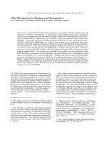
Figure 1: (a) A probabilistic FST defining a joint probability
distribution. (b) A smaller joint distribution. (c) A conditional
distribution. Defining (a)=(b)◦(c) means that the weights in (a)
can be altered by adjusting the fewer weights in (b) and (c).
This paper aims to provide a remedy through a
new paradigm, which we call parameterized finite-
state machines. It lays out a fully general approach
for training the weights of weighted rational rela-
tions. First §2 considers how to parameterize such
models, so that weights are defined in terms of un-
derlying parameters to be learned. §3 asks what it
means to learn these parameters from training data
(what is to be optimized?), and notes the apparently
formidable bookkeeping involved. §4 cuts through
the difficulty with a surprisingly simple trick. Fi-
nally, §5 removes inefficiencies from the basic algo-
rithm, making it suitable for inclusion in an actual
toolkit. Such a toolkit could greatly shorten the de-
velopment cycle in natural language engineering.
2 Transducers and Parameters
Finite-state machines, including finite-state au-
tomata (FSAs) and transducers (FSTs), are a kind
of labeled directed multigraph. For ease and brevity,
we explain them by example. Fig. 1a shows a proba-
bilistic FST with input alphabet Σ = {a, b}, output

alphabet ∆ = {x, z}, and all states final. It may
be regarded as a device for generating a string pair
in Σ
∗
× ∆
∗
by a random walk from
0


. Two paths
exist that generate both input aabb and output xz:
0


a:x/.63
−→
0
a:/.07
−→
1
b:/.03
−→
2
b:z/.4
−→
2/.5

0



a:x/.63
−→
0
a:/.07
−→
1
b:z/.12
−→
2
b:/.1
−→
2/.5

Each of the paths has probability .0002646, so
the probability of somehow generating the pair
(aabb, xz) is .0002646 + .0002646 = .0005292.
Abstracting away from the idea of random walks,
arc weights need not be probabilities. Still, define a
path’s weight as the product of its arc weights and
the stopping weight of its final state. Thus Fig. 1a
defines a weighted relation f where f(aabb, xz) =
.0005292. This particular relation does happen to be
probabilistic (see §1). It represents a joint distribu-
tion (since

x,y
f(x, y) = 1). Meanwhile, Fig. 1c
defines a conditional one (∀x


y
f(x, y) = 1).
This paper explains how to adjust probability dis-
tributions like that of Fig. 1a so as to model training
data better. The algorithm improves an FST’s nu-
meric weights while leaving its topology fixed.
How many parameters are there to adjust in
Fig. 1a? That is up to the user who built it! An
FST model with few parameters is more constrained,
making optimization easier. Some possibilities:
• Most simply, the algorithm can be asked to tune
the 17 numbers in Fig. 1a separately, subject to the
constraint that the paths retain total probability 1. A
more specific version of the constraint requires the
FST to remain Markovian: each of the 4 states must
present options with total probability 1 (at state
1
,
15+.7+.03.+.12=1). This preserves the random-walk
interpretation and (we will show) entails no loss of
generality. The 4 restrictions leave 13 free params.
• But perhaps Fig. 1a was actually obtained as
the composition of Fig. 1b–c, effectively defin-
ing P (input, output) =

mid
P (input, mid) ·
P (output | mid). If Fig. 1b–c are required to re-
main Markovian, they have 5 and 1 degrees of free-
dom respectively, so now Fig. 1a has only 6 param-

eters total.
2
In general, composing machines mul-
tiplies their arc counts but only adds their param-
eter counts. We wish to optimize just the few un-
derlying parameters, not independently optimize the
many arc weights of the composed machine.
• Perhaps Fig. 1b was itself obtained by the proba-
bilistic regular expression (a : p)∗
λ
(b : (p +
µ
q))∗
ν
with the 3 parameters (λ, µ, ν) = (.7, .2, .5). With
ρ = .1 from footnote 2, the composed machine
2
Why does Fig. 1c have only 1 degree of freedom? The
Markovian requirement means something different in Fig. 1c,
which defines a conditional relation P (output | mid) rather
than a joint one. A random walk on Fig. 1c chooses among arcs
with a given input label. So the arcs from state
6
with input
p must have total probability 1 (currently .9+.1). All other arc
choices are forced by the input label and so have probability 1.
The only tunable value is .1 (denote it by ρ), with .9 = 1 − ρ.
(Fig. 1a) has now been described with a total of just
4 parameters!
3

Here, probabilistic union E +
µ
F
def
=
µE + (1 − µ)F means “flip a µ-weighted coin and
generate E if heads, F if tails.” E∗
λ
def
= (λE)
∗
(1−λ)
means “repeatedly flip an λ-weighted coin and keep
repeating E as long as it comes up heads.”
These 4 parameters have global effects on Fig. 1a,
thanks to complex parameter tying: arcs
4
b:p
−→
5
,
5
b:q
−→
5
in Fig. 1b get respective probabilities (1 −
λ)µν and (1 − µ)ν, which covary with ν and vary
oppositely with µ. Each of these probabilities in turn
affects multiple arcs in the composed FST of Fig. 1a.
We offer a theorem that highlights the broad

applicability of these modeling techniques.
4
If
f(input, output) is a weighted regular relation,
then the following statements are equivalent: (1) f is
a joint probabilistic relation; (2) f can be computed
by a Markovian FST that halts with probability 1;
(3) f can be expressed as a probabilistic regexp,
i.e., a regexp built up from atomic expressions a : b
(for a ∈ Σ ∪ {}, b ∈ ∆ ∪ {}) using concatenation,
probabilistic union +
p
, and probabilistic closure ∗
p
.
For defining conditional relations, a good regexp
language is unknown to us, but they can be defined
in several other ways: (1) via FSTs as in Fig. 1c, (2)
by compilation of weighted rewrite rules (Mohri and
Sproat, 1996), (3) by compilation of decision trees
(Sproat and Riley, 1996), (4) as a relation that per-
forms contextual left-to-right replacement of input
substrings by a smaller conditional relation (Gerde-
mann and van Noord, 1999),
5
(5) by conditionaliza-
tion of a joint relation as discussed below.
A central technique is to define a joint relation as a
noisy-channel model, by composing a joint relation
with a cascade of one or more conditional relations

as in Fig. 1 (Pereira and Riley, 1997; Knight and
Graehl, 1998). The general form is illustrated by
3
Conceptually, the parameters represent the probabilities of
reading another a (λ); reading another b (ν); transducing b to p
rather than q (µ); starting to transduce p to  rather than x (ρ).
4
To prove (1)⇒(3), express f as an FST and apply the
well-known Kleene-Sch
¨
utzenberger construction (Berstel and
Reutenauer, 1988), taking care to write each regexp in the con-
struction as a constant times a probabilistic regexp. A full proof
is straightforward, as are proofs of (3)⇒(2), (2)⇒(1).
5
In (4), the randomness is in the smaller relation’s choice of
how to replace a match. One can also get randomness through
the choice of matches, ignoring match possibilities by randomly
deleting markers in Gerdemann and van Noord’s construction.
P (v, z)
def
=

w,x,y
P (v|w)P (w, x)P (y|x)P (z|y),
implemented by composing 4 machines.
6,7
There are also procedures for defining weighted
FSTs that are not probabilistic (Berstel and
Reutenauer, 1988). Arbitrary weights such as 2.7

may be assigned to arcs or sprinkled through a reg-
exp (to be compiled into
:/2.7
−→
arcs). A more subtle
example is weighted FSAs that approximate PCFGs
(Nederhof, 2000; Mohri and Nederhof, 2001), or
to extend the idea, weighted FSTs that approximate
joint or conditional synchronous PCFGs built for
translation. These are parameterized by the PCFG’s
parameters, but add or remove strings of the PCFG
to leave an improper probability distribution.
Fortunately for those techniques, an FST with
positive arc weights can be normalized to make it
jointly or conditionally probabilistic:
• An easy approach is to normalize the options at
each state to make the FST Markovian. Unfortu-
nately, the result may differ for equivalent FSTs that
express the same weighted relation. Undesirable
consequences of this fact have been termed “label
bias” (Lafferty et al., 2001). Also, in the conditional
case such per-state normalization is only correct if
all states accept all input suffixes (since “dead ends”
leak probability mass).
8
• A better-founded approach is global normal-
ization, which simply divides each f(x, y) by

x


,y

f(x

, y

) (joint case) or by

y

f(x, y

) (con-
ditional case). To implement the joint case, just di-
vide stopping weights by the total weight of all paths
(which §4 shows how to find), provided this is finite.
In the conditional case, let g be a copy of f with the
output labels removed, so that g(x) finds the desired
divisor; determinize g if possible (but this fails for
some weighted FSAs), replace all weights with their
reciprocals, and compose the result with f.
9
6
P (w, x) defines the source model, and is often an “identity
FST” that requires w = x, really just an FSA.
7
We propose also using n-tape automata to generalize to
“branching noisy channels” (a case of dendroid distributions).
In


w,x
P (v|w)P (v

|w)P (w, x)P (y|x), the true transcrip-
tion w can be triply constrained by observing speech y and two
errorful transcriptions v, v

, which independently depend on w.
8
A corresponding problem exists in the joint case, but may
be easily avoided there by first pruning non-coaccessible states.
9
It suffices to make g unambiguous (one accepting path per
string), a weaker condition than determinism. When this is not
possible (as in the inverse of Fig. 1b, whose conditionaliza-
Normalization is particularly important because it
enables the use of log-linear (maximum-entropy)
parameterizations. Here one defines each arc
weight, coin weight, or regexp weight in terms of
meaningful features associated by hand with that
arc, coin, etc. Each feature has a strength ∈ R
>0
,
and a weight is computed as the product of the
strengths of its features.
10
It is now the strengths
that are the learnable parameters. This allows mean-
ingful parameter tying: if certain arcs such as
u:i

−→
,
o:e
−→
, and
a:ae
−→
share a contextual “vowel-fronting”
feature, then their weights rise and fall together with
the strength of that feature. The resulting machine
must be normalized, either per-state or globally, to
obtain a joint or a conditional distribution as de-
sired. Such approaches have been tried recently
in restricted cases (McCallum et al., 2000; Eisner,
2001b; Lafferty et al., 2001).
Normalization may be postponed and applied in-
stead to the result of combining the FST with other
FSTs by composition, union, concatenation, etc. A
simple example is a probabilistic FSA defined by
normalizing the intersection of other probabilistic
FSAs f
1
, f
2
, . . (This is in fact a log-linear model
in which the component FSAs define the features:
string x has log f
i
(x) occurrences of feature i.)
In short, weighted finite-state operators provide a

language for specifying a wide variety of parameter-
ized statistical models. Let us turn to their training.
3 Estimation in Parameterized FSTs
We are primarily concerned with the following train-
ing paradigm, novel in its generality. Let f
θ
:
Σ
∗
×∆
∗
→ R
≥0
be a joint probabilistic relation that
is computed by a weighted FST. The FST was built
by some recipe that used the parameter vector θ.
Changing θ may require us to rebuild the FST to get
updated weights; this can involve composition, reg-
exp compilation, multiplication of feature strengths,
etc. (Lazy algorithms that compute arcs and states of
tion cannot be realized by any weighted FST), one can some-
times succeed by first intersecting g with a smaller regular set
in which the input being considered is known to fall. In the ex-
treme, if each input string is fully observed (not the case if the
input is bound by composition to the output of a one-to-many
FST), one can succeed by restricting g to each input string in
turn; this amounts to manually dividing f(x, y) by g(x).
10
Traditionally log(strength) values are called weights, but
this paper uses “weight” to mean something else.

8 9
a:x/.63
10
a:x/.63
11
b:x/.027
a: /.7ε
b: /.0051ε
12/.5
b:z/.1284
b: /.1ε b:z/.404
b: /.1ε
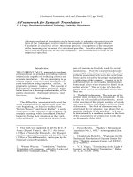
Figure 2: The joint model of Fig. 1a constrained to generate
only input ∈ a(a + b)
∗
and output = xxz.
f
θ
on demand (Mohri et al., 1998) can pay off here,
since only part of f
θ
may be needed subsequently.)
As training data we are given a set of observed
(input, output) pairs, (x
i
, y
i
). These are assumed
to be independent random samples from a joint dis-
tribution of the form f

ˆ
θ
(x, y); the goal is to recover
the true
ˆ
θ. Samples need not be fully observed
(partly supervised training): thus x
i
⊆ Σ
∗
, y
i
⊆ ∆
∗
may be given as regular sets in which input and out-
put were observed to fall. For example, in ordinary
HMM training, x
i
= Σ
∗
and represents a completely
hidden state sequence (cf. Ristad (1998), who allows
any regular set), while y
i
is a single string represent-
ing a completely observed emission sequence.
11
What to optimize? Maximum-likelihood es-
timation guesses
ˆ

θ to be the θ maximizing

i
f
θ
(x
i
, y
i
). Maximum-posterior estimation
tries to maximize P (θ)·

i
f
θ
(x
i
, y
i
) where P (θ) is
a prior probability. In a log-linear parameterization,
for example, a prior that penalizes feature strengths
far from 1 can be used to do feature selection and
avoid overfitting (Chen and Rosenfeld, 1999).
The EM algorithm (Dempster et al., 1977) can
maximize these functions. Roughly, the E step
guesses hidden information: if (x
i
, y
i

) was gener-
ated from the current f
θ
, which FST paths stand a
chance of having been the path used? (Guessing the
path also guesses the exact input and output.) The
M step updates θ to make those paths more likely.
EM alternates these steps and converges to a local
optimum. The M step’s form depends on the param-
eterization and the E step serves the M step’s needs.
Let f
θ
be Fig. 1a and suppose (x
i
, y
i
) = (a(a +
b)
∗
, xxz). During the E step, we restrict to paths
compatible with this observation by computing x
i
◦
f
θ
◦ y
i
, shown in Fig. 2. To find each path’s pos-
terior probability given the observation (x
i

, y
i
), just
conditionalize: divide its raw probability by the total
probability (≈ 0.1003) of all paths in Fig. 2.
11
To implement an HMM by an FST, compose a probabilistic
FSA that generates a state sequence of the HMM with a condi-
tional FST that transduces HMM states to emitted symbols.
But that is not the full E step. The M step uses
not individual path probabilities (Fig. 2 has infinitely
many) but expected counts derived from the paths.
Crucially, §4 will show how the E step can accumu-
late these counts effortlessly. We first explain their
use by the M step, repeating the presentation of §2:
• If the parameters are the 17 weights in Fig. 1a, the
M step reestimates the probabilities of the arcs from
each state to be proportional to the expected number
of traversals of each arc (normalizing at each state
to make the FST Markovian). So the E step must
count traversals. This requires mapping Fig. 2 back
onto Fig. 1a: to traverse either
8
a:x
−→
9
or
9
a:x
−→

10
in Fig. 2 is “really” to traverse
0
a:x
−→
0
in Fig. 1a.
• If Fig. 1a was built by composition, the M step
is similar but needs the expected traversals of the
arcs in Fig. 1b–c. This requires further unwinding of
Fig. 1a’s
0
a:x
−→
0
: to traverse that arc is “really” to
traverse Fig. 1b’s
4
a:p
−→
4
and Fig. 1c’s
6
p:x
−→
6
.
• If Fig. 1b was defined by the regexp given earlier,
traversing
4

a:p
−→
4
is in turn “really” just evidence
that the λ-coin came up heads. To learn the weights
λ, ν, µ, ρ, count expected heads/tails for each coin.
• If arc probabilities (or even λ, ν, µ, ρ) have log-
linear parameterization, then the E step must com-
pute c =

i
ec
f
(x
i
, y
i
), where ec(x, y) denotes
the expected vector of total feature counts along a
random path in f
θ
whose (input, output) matches
(x, y). The M step then treats c as fixed, observed
data and adjusts θ until the predicted vector of to-
tal feature counts equals c, using Improved Itera-
tive Scaling (Della Pietra et al., 1997; Chen and
Rosenfeld, 1999).
12
For globally normalized, joint
models, the predicted vector is ec

f
(Σ
∗
, ∆
∗
). If the
log-linear probabilities are conditioned on the state
and/or the input, the predicted vector is harder to de-
scribe (though usually much easier to compute).
13
12
IIS is itself iterative; to avoid nested loops, run only one it-
eration at each M step, giving a GEM algorithm (Riezler, 1999).
Alternatively, discard EM and use gradient-based optimization.
13
For per-state conditional normalization, let D
j,a
be the set
of arcs from state j with input symbol a ∈ Σ; their weights are
normalized to sum to 1. Besides computing c, the E step must
count the expected number d
j,a
of traversals of arcs in each
D
j,a
. Then the predicted vector given θ is

j,a
d
j,a

·(expected
feature counts on a randomly chosen arc in D
j,a
). Per-state
joint normalization (Eisner, 2001b, §8.2) is similar but drops the
dependence on a. The difficult case is global conditional nor-
malization. It arises, for example, when training a joint model
of the form f
θ
= · · · (g
θ
◦ h
θ
) · · ·, where h
θ
is a conditional
It is also possible to use this EM approach for dis-
criminative training, where we wish to maximize

i
P (y
i
| x
i
) and f
θ
(x, y) is a conditional FST that
defines P (y | x). The trick is to instead train a joint
model g ◦ f
θ

, where g(x
i
) defines P (x
i
), thereby
maximizing

i
P (x
i
) · P (y
i
| x
i
). (Of course,
the method of this paper can train such composi-
tions.) If x
1
, . . . x
n
are fully observed, just define
each g(x
i
) = 1/n. But by choosing a more gen-
eral model of g, we can also handle incompletely
observed x
i
: training g ◦ f
θ
then forces g and f

θ
to cooperatively reconstruct a distribution over the
possible inputs and do discriminative training of f
θ
given those inputs. (Any parameters of g may be ei-
ther frozen before training or optimized along with
the parameters of f
θ
.) A final possibility is that each
x
i
is defined by a probabilistic FSA that already sup-
plies a distribution over the inputs; then we consider
x
i
◦ f
θ
◦ y
i
directly, just as in the joint model.
Finally, note that EM is not all-purpose. It only
maximizes probabilistic objective functions, and
even there it is not necessarily as fast as (say) conju-
gate gradient. For this reason, we will also show be-
low how to compute the gradient of f
θ
(x
i
, y
i

) with
respect to θ, for an arbitrary parameterized FST f
θ
.
We remark without elaboration that this can help
optimize task-related objective functions, such as

i

y
(P (x
i
, y)
α
/

y

P (x
i
, y

)
α
) · error(y, y
i
).
4 The E Step: Expectation Semirings
It remains to devise appropriate E steps, which looks
rather daunting. Each path in Fig. 2 weaves together

parameters from other machines, which we must un-
tangle and tally. In the 4-coin parameterization, path
8


a:x
−→
9
a:x
−→
10
a:
−→
10
a:
−→
10
b:z
−→
12
must yield up a
vector H
λ
, T
λ
, H
µ
, T
µ
, H

ν
, T
ν
, H
ρ
, T
ρ
 that counts
observed heads and tails of the 4 coins. This non-
trivially works out to 4, 1, 0, 1, 1, 1, 1, 2. For other
parameterizations, the path must instead yield a vec-
tor of arc traversal counts or feature counts.
Computing a count vector for one path is hard
enough, but it is the E step’s job to find the expected
value of this vector—an average over the infinitely
log-linear model of P (v | u) for u ∈ Σ
∗
, v ∈ ∆
∗
. Then the
predicted count vector contributed by h is

i

u∈Σ
∗
P (u |
x
i
, y

i
) · ec
h
(u, ∆
∗
). The term

i
P (u | x
i
, y
i
) computes the
expected count of each u ∈ Σ
∗
. It may be found by a variant
of §4 in which path values are regular expressions over Σ
∗
.
many paths π through Fig. 2 in proportion to their
posterior probabilities P(π | x
i
, y
i
). The results for
all (x
i
, y
i
) are summed and passed to the M step.

Abstractly, let us say that each path π has not only
a probability P (π) ∈ [0, 1] but also a value val(π)
in a vector space V , which counts the arcs, features,
or coin flips encountered along path π. The value of
a path is the sum of the values assigned to its arcs.
The E step must return the expected value of the
unknown path that generated (x
i
, y
i
). For example,
if every arc had value 1, then expected value would
be expected path length. Letting Π denote the set of
paths in x
i
◦ f
θ
◦ y
i
(Fig. 2), the expected value is
14
E[val(π) | x
i
, y
i
] =

π∈Π
P (π) val(π)


π∈Π
P (π)
(1)
The denominator of equation (1) is the total prob-
ability of all accepting paths in x
i
◦ f ◦ y
i
. But while
computing this, we will also compute the numerator.
The idea is to augment the weight data structure with
expectation information, so each weight records a
probability and a vector counting the parameters
that contributed to that probability. We will enforce
an invariant: the weight of any pathset Π must
be (

π∈Π
P (π),

π∈Π
P (π) val(π)) ∈ R
≥0
× V ,
from which (1) is trivial to compute.
Berstel and Reutenauer (1988) give a sufficiently
general finite-state framework to allow this: weights
may fall in any set K (instead of R). Multiplica-
tion and addition are replaced by binary operations
⊗ and ⊕ on K. Thus ⊗ is used to combine arc

weights into a path weight and ⊕ is used to com-
bine the weights of alternative paths. To sum over
infinite sets of cyclic paths we also need a closure
operation
∗
, interpreted as k
∗
=

∞
i=0
k
i
. The usual
finite-state algorithms work if (K, ⊕, ⊗,
∗
) has the
structure of a closed semiring.
15
Ordinary probabilities fall in the semiring
(R
≥0
, +, ×,
∗
).
16
Our novel weights fall in a novel
14
Formal derivation of (1):


π
P (π | x
i
, y
i
) val(π) =
(

π
P (π, x
i
, y
i
) val(π))/P (x
i
, y
i
) = (

π
P (x
i
, y
i
|
π)P(π) val(π))/

π
P (x
i

, y
i
| π)P (π); now observe that
P (x
i
, y
i
| π) = 1 or 0 according to whether π ∈ Π.
15
That is: (K, ⊗) is a monoid (i.e., ⊗ : K × K → K is
associative) with identity 1. (K, ⊕) is a commutative monoid
with identity 0. ⊗ distributes over ⊕ from both sides, 0 ⊗ k =
k ⊗ 0 = 0, and k
∗
= 1 ⊕ k ⊗ k
∗
= 1 ⊕ k
∗
⊗ k. For finite-state
composition, commutativity of ⊗ is needed as well.
16
The closure operation is defined for p ∈ [0, 1) as p
∗
=
1/(1 − p), so cycles with weights in [0, 1) are allowed.
V -expectation semiring, (R
≥0
× V, ⊕, ⊗,
∗
):

(p
1
, v
1
) ⊗ (p
2
, v
2
)
def
= (p
1
p
2
, p
1
v
2
+ v
1
p
2
) (2)
(p
1
, v
1
) ⊕ (p
2
, v

2
)
def
= (p
1
+ p
2
, v
1
+ v
2
) (3)
if p
∗
defined, (p, v)
∗
def
= (p
∗
, p
∗
vp
∗
) (4)
If an arc has probability p and value v, we give it
the weight (p, pv), so that our invariant (see above)
holds if Π consists of a single length-0 or length-1
path. The above definitions are designed to preserve
our invariant as we build up larger paths and path-
sets. ⊗ lets us concatenate (e.g.) simple paths π

1
, π
2
to get a longer path π with P (π) = P(π
1
)P (π
2
)
and val(π) = val(π
1
) + val(π
2
). The defini-
tion of ⊗ guarantees that path π’s weight will be
(P (π), P(π) · val(π)). ⊕ lets us take the union of
two disjoint pathsets, and
∗
computes infinite unions.
To compute (1) now, we only need the total
weight t
i
of accepting paths in x
i
◦ f ◦ y
i
(Fig. 2).
This can be computed with finite-state methods: the
machine (×x
i
)◦f ◦(y

i
×) is a version that replaces
all input:output labels with  : , so it maps (, ) to
the same total weight t
i
. Minimizing it yields a one-
state FST from which t
i
can be read directly!
The other “magical” property of the expecta-
tion semiring is that it automatically keeps track of
the tangled parameter counts. For instance, recall
that traversing
0
a:x
−→
0
should have the same ef-
fect as traversing both the underlying arcs
4
a:p
−→
4
and
6
p:x
−→
6
. And indeed, if the underlying arcs
have values v

1
and v
2
, then the composed arc
0
a:x
−→
0
gets weight (p
1
, p
1
v
1
) ⊗ (p
2
, p
2
v
2
) =
(p
1
p
2
, p
1
p
2
(v

1
+ v
2
)), just as if it had value v
1
+ v
2
.
Some concrete examples of values may be useful:
• To count traversals of the arcs of Figs. 1b–c, num-
ber these arcs and let arc  have value e

, the 
th
basis
vector. Then the 
th
element of val(π) counts the ap-
pearances of arc  in path π, or underlying path π.
• A regexp of form E+
µ
F = µE+(1−µ)F should
be weighted as (µ, µe
k
)E + (1 − µ, (1 − µ)e
k+1
)F
in the new semiring. Then elements k and k + 1 of
val(π) count the heads and tails of the µ-coin.
• For a global log-linear parameterization, an arc’s

value is a vector specifying the arc’s features. Then
val(π) counts all the features encountered along π.
Really we are manipulating weighted relations,
not FSTs. We may combine FSTs, or determinize
or minimize them, with any variant of the semiring-
weighted algorithms.
17
As long as the resulting FST
computes the right weighted relation, the arrange-
ment of its states, arcs, and labels is unimportant.
The same semiring may be used to compute gradi-
ents. We would like to find f
θ
(x
i
, y
i
) and its gradient
with respect to θ, where f
θ
is real-valued but need
not be probabilistic. Whatever procedures are used
to evaluate f
θ
(x
i
, y
i
) exactly or approximately—for
example, FST operations to compile f

θ
followed by
minimization of ( × x
i
) ◦ f
θ
◦ (y
i
× )—can simply
be applied over the expectation semiring, replacing
each weight p by (p, ∇p) and replacing the usual
arithmetic operations with ⊕, ⊗, etc.
18
(2)–(4) pre-
serve the gradient ((2) is the derivative product rule),
so this computation yields (f
θ
(x
i
, y
i
), ∇f
θ
(x
i
, y
i
)).
5 Removing Inefficiencies
Now for some important remarks on efficiency:

• Computing t
i
is an instance of the well-known
algebraic path problem (Lehmann, 1977; Tarjan,
1981a). Let T
i
= x
i
◦f ◦y
i
. Then t
i
is the total semir-
ing weight w
0n
of paths in T
i
from initial state 0 to
final state n (assumed WLOG to be unique and un-
weighted). It is wasteful to compute t
i
as suggested
earlier, by minimizing (×x
i
)◦f ◦(y
i
×), since then
the real work is done by an -closure step (Mohri,
2002) that implements the all-pairs version of alge-
braic path, whereas all we need is the single-source

version. If n and m are the number of states and
edges,
19
then both problems are O(n
3
) in the worst
case, but the single-source version can be solved in
essentially O(m) time for acyclic graphs and other
reducible flow graphs (Tarjan, 1981b). For a gen-
eral graph T
i
, Tarjan (1981b) shows how to partition
into “hard” subgraphs that localize the cyclicity or
irreducibility, then run the O(n
3
) algorithm on each
subgraph (thereby reducing n to as little as 1), and
recombine the results. The overhead of partitioning
and recombining is essentially only O(m).
• For speeding up the O(n
3
) problem on subgraphs,
one can use an approximate relaxation technique
17
Eisner (submitted) develops fast minimization algorithms
that work for the real and V -expectation semirings.
18
Division and subtraction are also possible: −(p, v) =
(−p, −v) and (p, v)
−1

= (p
−1
, −p
−1
vp
−1
). Division is com-
monly used in defining f
θ
(for normalization).
19
Multiple edges from j to k are summed into a single edge.
(Mohri, 2002). Efficient hardware implementation is
also possible via chip-level parallelism (Rote, 1985).
• In many cases of interest, T
i
is an acyclic graph.
20
Then Tarjan’s method computes w
0j
for each j in
topologically sorted order, thereby finding t
i
in a
linear number of ⊕ and ⊗ operations. For HMMs
(footnote 11), T
i
is the familiar trellis, and we would
like this computation of t
i

to reduce to the forward-
backward algorithm (Baum, 1972). But notice that
it has no backward pass. In place of pushing cumu-
lative probabilities backward to the arcs, it pushes
cumulative arcs (more generally, values in V ) for-
ward to the probabilities. This is slower because
our ⊕ and ⊗ are vector operations, and the vec-
tors rapidly lose sparsity as they are added together.
We therefore reintroduce a backward pass that lets
us avoid ⊕ and ⊗ when computing t
i
(so they are
needed only to construct T
i
). This speedup also
works for cyclic graphs and for any V . Write w
jk
as (p
jk
, v
jk
), and let w
1
jk
= (p
1
jk
, v
1
jk

) denote the
weight of the edge from j to k.
19
Then it can be
shown that w
0n
= (p
0n
,

j,k
p
0j
v
1
jk
p
kn
). The for-
ward and backward probabilities, p
0j
and p
kn
, can
be computed using single-source algebraic path for
the simpler semiring (R, +, ×,
∗
)—or equivalently,
by solving a sparse linear system of equations over
R, a much-studied problem at O(n) space, O(nm)

time, and faster approximations (Greenbaum, 1997).
• A Viterbi variant of the expectation semiring ex-
ists: replace (3) with if(p
1
> p
2
, (p
1
, v
1
), (p
2
, v
2
)).
Here, the forward and backward probabilities can be
computed in time only O(m + n log n) (Fredman
and Tarjan, 1987). k-best variants are also possible.
6 Discussion
We have exhibited a training algorithm for param-
eterized finite-state machines. Some specific conse-
quences that we believe to be novel are (1) an EM al-
gorithm for FSTs with cycles and epsilons; (2) train-
ing algorithms for HMMs and weighted contextual
edit distance that work on incomplete data; (3) end-
to-end training of noisy channel cascades, so that it
is not necessary to have separate training data for
each machine in the cascade (cf. Knight and Graehl,
20
If x

i
and y
i
are acyclic (e.g., fully observed strings), and
f (or rather its FST) has no  :  cycles, then composition will
“unroll” f into an acyclic machine. If only x
i
is acyclic, then
the composition is still acyclic if domain(f) has no  cycles.
1998), although such data could also be used; (4)
training of branching noisy channels (footnote 7);
(5) discriminative training with incomplete data; (6)
training of conditional MEMMs (McCallum et al.,
2000) and conditional random fields (Lafferty et al.,
2001) on unbounded sequences.
We are particularly interested in the potential for
quickly building statistical models that incorporate
linguistic and engineering insights. Many models of
interest can be constructed in our paradigm, without
having to write new code. Bringing diverse models
into the same declarative framework also allows one
to apply new optimization methods, objective func-
tions, and finite-state algorithms to all of them.
To avoid local maxima, one might try determinis-
tic annealing (Rao and Rose, 2001), or randomized
methods, or place a prior on θ. Another extension is
to adjust the machine topology, say by model merg-
ing (Stolcke and Omohundro, 1994). Such tech-
niques build on our parameter estimation method.
The key algorithmic ideas of this paper extend

from forward-backward-style to inside-outside-style
methods. For example, it should be possible to do
end-to-end training of a weighted relation defined
by an interestingly parameterized synchronous CFG
composed with tree transducers and then FSTs.
References
L. E. Baum. 1972. An inequality and associated max-
imization technique in statistical estimation of proba-
bilistic functions of a Markov process. Inequalities, 3.
Jean Berstel and Christophe Reutenauer. 1988. Rational
Series and their Languages. Springer-Verlag.
Stanley F. Chen and Ronald Rosenfeld. 1999. A Gaus-
sian prior for smoothing maximum entropy models.
Technical Report CMU-CS-99-108, Carnegie Mellon.
S. Della Pietra, V. Della Pietra, and J. Lafferty. 1997.
Inducing features of random fields. IEEE Transactions
on Pattern Analysis and Machine Intelligence, 19(4).
A. P. Dempster, N. M. Laird, and D. B. Rubin. 1977.
Maximum likelihood from incomplete data via the EM
algorithm. J. Royal Statist. Soc. Ser. B, 39(1):1–38.
Jason Eisner. 2001a. Expectation semirings: Flexible
EM for finite-state transducers. In G. van Noord, ed.,
Proc. of the ESSLLI Workshop on Finite-State Methods
in Natural Language Processing. Extended abstract.
Jason Eisner. 2001b. Smoothing a Probabilistic Lexicon
via Syntactic Transformations. Ph.D. thesis, Univer-
sity of Pennsylvania.
D. Gerdemann and G. van Noord. 1999. Transducers
from rewrite rules with backreferences. Proc. of EACL.
Anne Greenbaum. 1997. Iterative Methods for Solving

Linear Systems. Soc. for Industrial and Applied Math.
Kevin Knight and Yaser Al-Onaizan. 1998. Translation
with finite-state devices. In Proc. of AMTA.
Kevin Knight and Jonathan Graehl. 1998. Machine
transliteration. Computational Linguistics, 24(4).
J. Lafferty, A. McCallum, and F. Pereira. 2001. Con-
ditional random fields: Probabilistic models for seg-
menting and labeling sequence data. Proc. of ICML.
D. J. Lehmann. 1977. Algebraic structures for transitive
closure. Theoretical Computer Science, 4(1):59–76.
A. McCallum, D. Freitag, and F. Pereira. 2000. Maxi-
mum entropy Markov models for information extrac-
tion and segmentation. Proc. of ICML, 591–598.
M. Mohri and M J. Nederhof. 2001. Regular approxi-
mation of context-free grammars through transforma-
tion. In J C. Junqua and G. van Noord, eds., Robust-
ness in Language and Speech Technology. Kluwer.
Mehryar Mohri and Richard Sproat. 1996. An efficient
compiler for weighted rewrite rules. In Proc. of ACL.
M. Mohri, F. Pereira, and M. Riley. 1998. A rational de-
sign for a weighted finite-state transducer library. Lec-
ture Notes in Computer Science, 1436.
M. Mohri. 2002. Generic epsilon-removal and input
epsilon-normalization algorithms for weighted trans-
ducers. Int. J. of Foundations of Comp. Sci., 1(13).
Mark-Jan Nederhof. 2000. Practical experiments
with regular approximation of context-free languages.
Computational Linguistics, 26(1).
Fernando C. N. Pereira and Michael Riley. 1997. Speech
recognition by composition of weighted finite au-

tomata. In E. Roche and Y. Schabes, eds., Finite-State
Language Processing. MIT Press, Cambridge, MA.
A. Rao and K. Rose. 2001 Deterministically annealed
design of hidden Markov movel speech recognizers.
In IEEE Trans. on Speech and Audio Processing, 9(2).
Stefan Riezler. 1999. Probabilistic Constraint Logic
Programming. Ph.D. thesis, Universit
¨
at T
¨
ubingen.
E. Ristad and P. Yianilos. 1996. Learning string edit
distance. Tech. Report CS-TR-532-96, Princeton.
E. Ristad. 1998. Hidden Markov models with finite state
supervision. In A. Kornai, ed., Extended Finite State
Models of Language. Cambridge University Press.
Emmanuel Roche and Yves Schabes, editors. 1997.
Finite-State Language Processing. MIT Press.
G
¨
unter Rote. 1985. A systolic array algorithm for the
algebraic path problem (shortest paths; matrix inver-
sion). Computing, 34(3):191–219.
Richard Sproat and Michael Riley. 1996. Compilation of
weighted finite-state transducers from decision trees.
In Proceedings of the 34th Annual Meeting of the ACL.
Andreas Stolcke and Stephen M. Omohundro. 1994.
Best-first model merging for hidden Markov model in-
duction. Tech. Report ICSI TR-94-003, Berkeley, CA.
Robert Endre Tarjan. 1981a. A unified approach to path

problems. Journal of the ACM, 28(3):577–593, July.
Robert Endre Tarjan. 1981b. Fast algorithms for solving
path problems. J. of the ACM, 28(3):594–614, July.
G. van Noord and D. Gerdemann. 2001. An extendible
regular expression compiler for finite-state approaches
in natural language processing. In Automata Imple-
mentation, no. 22 in Springer Lecture Notes in CS.