Ron larson, robert p hostetler, bruce h edwards calculus early transcendental functions, fourth edition cengage learning (2006)

Calculus
Early Transcendental Functions
Fourth Edition

Ron Larson
The Pennsylvania State University
The Behrend College

Robert Hostetler
The Pennsylvania State University
The Behrend College

Bruce H. Edwards
University of Florida

Houghton Mifflin Company

Boston

New York


Publisher: Richard Stratton
Sponsoring Editor: Cathy Cantin
Development Manager: Maureen Ross
Associate Editor: Yen Tieu
Editorial Associate: Elizabeth Kassab
Supervising Editor: Karen Carter
Senior Project Editor: Patty Bergin
Editorial Assistant: Julia Keller

Art and Design Manager: Gary Crespo
Executive Marketing Manager: Brenda Bravener-Greville
Senior Marketing Manager: Danielle Curran
Director of Manufacturing: Priscilla Manchester
Cover Design Manager: Tony Saizon

We have included examples and exercises that use real-life data as well as technology output from a variety of software. This would not have been possible without the help of many
people and organizations. Our wholehearted thanks goes to all for their time and effort.
Cover photograph: “Music of the Spheres” by English sculptor John Robinson is a
three-foot-tall sculpture in bronze that has one continuous edge. You can trace its edge
three times around before returning to the starting point. To learn more about this and other
works by John Robinson, see the Centre for the Popularisation of Mathematics, University
of Wales, at />Trademark Acknowledgments: TI is a registered trademark of Texas Instruments, Inc.
Mathcad is a registered trademark of MathSoft, Inc. Windows, Microsoft, and MS-DOS are
registered trademarks of Microsoft, Inc. Mathematica is a registered trademark of Wolfram
Research, Inc. DERIVE is a registered trademark of Texas Instruments, Inc. IBM is a
registered trademark of International Business Machines Corporation. Maple is a registered
trademark of Waterloo Maple, Inc. HM ClassPrep is a trademark of Houghton Mifflin
Company. Diploma is a registered trademark of Brownstone Research Group.
Copyright © 2007 by Houghton Mifflin Company. All rights reserved.
No part of this work may be reproduced or transmitted in any form or by any means,
electronic or mechanical, including photocopying and recording, or by any information
storage or retrieval system, without the prior written permission of Houghton Mifflin
Company unless such copying is expressly permitted by federal copyright law. Address
inquiries to College Permissions, Houghton Mifflin Company, 222 Berkeley Street, Boston,
MA 02116-3764.
Printed in the U.S.A.
Library of Congress Control Number: 2005933918
Instructor’s exam copy:
ISBN 13: 978-0-618-73069-8

ISBN 10: 0-618-73069-9
For orders, use student text ISBNs:
ISBN 13: 978-0-618-60624-5
ISBN 10: 0-618-60624-6
1 2 3 4 5 6 7 8 9-DOW-10-09 08 07 06


Contents
A Word from the Authors
x
Integrated Learning System for Calculus
Features
xviii

Chapter 1

Preparation for Calculus

xii

I

1.1
1.2
1.3
1.4
1.5
1.6

Graphs and Models

2
Linear Models and Rates of Change
10
Functions and Their Graphs
19
Fitting Models to Data
31
Inverse Functions
37
Exponential and Logarithmic Functions
49
Review Exercises
57
P.S. Problem Solving
59

Chapter 2

Limits and Their Properties

61

2.1 A Preview of Calculus
62
2.2 Finding Limits Graphically and Numerically
68
2.3 Evaluating Limits Analytically
79
2.4 Continuity and One-Sided Limits
90

2.5 Infinite Limits
103
Section Project: Graphs and Limits of Trigonometric
Functions
110
Review Exercises
111
P.S. Problem Solving
113

Chapter 3

Differentiation

115

3.1 The Derivative and the Tangent Line Problem
116
3.2 Basic Differentiation Rules and Rates of Change
127
3.3 Product and Quotient Rules and Higher-Order
Derivatives
140
3.4 The Chain Rule
151
3.5 Implicit Differentiation
166
Section Project: Optical Illusions
174

iii


iv

CONTENTS

3.6 Derivatives of Inverse Functions
3.7 Related Rates
182
3.8 Newton’s Method
191
Review Exercises
197
P.S. Problem Solving
201

Chapter 4

Applications of Differentiation

175

203

4.1 Extrema on an Interval
204
4.2 Rolle’s Theorem and the Mean Value Theorem
212
4.3 Increasing and Decreasing Functions and the

First Derivative Test
219
Section Project: Rainbows
229
4.4 Concavity and the Second Derivative Test
230
4.5 Limits at Infinity
238
4.6 A Summary of Curve Sketching
249
4.7 Optimization Problems
259
Section Project: Connecticut River
270
4.8 Differentials
271
Review Exercises
278
P.S. Problem Solving
281

Chapter 5

Integration

283

5.1 Antiderivatives and Indefinite Integration
284
5.2 Area

295
5.3 Riemann Sums and Definite Integrals
307
5.4 The Fundamental Theorem of Calculus
318
Section Project: Demonstrating the Fundamental Theorem
5.5 Integration by Substitution
331
5.6 Numerical Integration
345
5.7 The Natural Logarithmic Function: Integration
352
5.8 Inverse Trigonometric Functions: Integration
361
5.9 Hyperbolic Functions
369
Section Project: St. Louis Arch
379
Review Exercises
380
P.S. Problem Solving
383

330


CONTENTS

Chapter 6

Differential Equations

v

385

6.1 Slope Fields and Euler’s Method
386
6.2 Differential Equations: Growth and Decay
395
6.3 Differential Equations: Separation of Variables
403
6.4 The Logistic Equation
417
6.5 First-Order Linear Differential Equations
424
Section Project: Weight Loss
432
6.6 Predator-Prey Differential Equations
433
Review Exercises
440
P.S. Problem Solving
443

Chapter 7

Applications of Integration

445

7.1 Area of a Region Between Two Curves
446
7.2 Volume: The Disk Method
456
7.3 Volume: The Shell Method
467
Section Project: Saturn
475
7.4 Arc Length and Surfaces of Revolution
476
7.5 Work
487
Section Project: Tidal Energy
495
7.6 Moments, Centers of Mass, and Centroids
496
7.7 Fluid Pressure and Fluid Force
507
Review Exercises
513
P.S. Problem Solving
515

Chapter 8

Integration Techniques, L’Hôpital’s Rule,
and Improper Integrals
517
8.1 Basic Integration Rules

518
8.2 Integration by Parts
525
8.3 Trigonometric Integrals
534
Section Project: Power Lines
542
8.4 Trigonometric Substitution
543
8.5 Partial Fractions
552
8.6 Integration by Tables and Other Integration Techniques
8.7 Indeterminate Forms and L’Hôpital’s Rule
567
8.8 Improper Integrals
578
Review Exercises
589
P.S. Problem Solving
591

561


vi

CONTENTS

Chapter 9

Infinite Series

593

9.1 Sequences
594
9.2 Series and Convergence
606
Section Project: Cantor’s Disappearing Table
616
9.3 The Integral Test and p-Series
617
Section Project: The Harmonic Series
623
9.4 Comparisons of Series
624
Section Project: Solera Method
630
9.5 Alternating Series
631
9.6 The Ratio and Root Tests
639
9.7 Taylor Polynomials and Approximations
648
9.8 Power Series
659
9.9 Representation of Functions by Power Series
669
9.10 Taylor and Maclaurin Series
676

Review Exercises
688
P.S. Problem Solving
691

Chapter 10

Conics, Parametric Equations, and
Polar Coordinates
693
10.1 Conics and Calculus
694
10.2 Plane Curves and Parametric Equations
709
Section Project: Cycloids
718
10.3 Parametric Equations and Calculus
719
10.4 Polar Coordinates and Polar Graphs
729
Section Project: Anamorphic Art
738
10.5 Area and Arc Length in Polar Coordinates
739
10.6 Polar Equations of Conics and Kepler’s Laws
748
Review Exercises
756
P.S. Problem Solving
759

CONTENTS

Chapter 11

Vectors and the Geometry of Space

vii

761

11.1 Vectors in the Plane
762
11.2 Space Coordinates and Vectors in Space
773
11.3 The Dot Product of Two Vectors
781
11.4 The Cross Product of Two Vectors in Space
790
11.5 Lines and Planes in Space
798
Section Project: Distances in Space
809
11.6 Surfaces in Space
810
11.7 Cylindrical and Spherical Coordinates
820
Review Exercises
827

P.S. Problem Solving
829

Chapter 12

Vector-Valued Functions

831

12.1 Vector-Valued Functions
832
Section Project: Witch of Agnesi
839
12.2 Differentiation and Integration of Vector-Valued
Functions
840
12.3 Velocity and Acceleration
848
12.4 Tangent Vectors and Normal Vectors
857
12.5 Arc Length and Curvature
867
Review Exercises
879
P.S. Problem Solving
881

Chapter 13

Functions of Several Variables

883

13.1 Introduction to Functions of Several Variables
884
13.2 Limits and Continuity
896
13.3 Partial Derivatives
906
Section Project: Moiré Fringes
915
13.4 Differentials
916
13.5 Chain Rules for Functions of Several Variables
923
13.6 Directional Derivatives and Gradients
931
13.7 Tangent Planes and Normal Lines
943
Section Project: Wildflowers
951
13.8 Extrema of Functions of Two Variables
952
13.9 Applications of Extrema of Functions of Two Variables
Section Project: Building a Pipeline
967
13.10 Lagrange Multipliers
968
Review Exercises
976

P.S. Problem Solving
979

960


viii

CONTENTS

Chapter 14

Multiple Integration

981

14.1 Iterated Integrals and Area in the Plane
982
14.2 Double Integrals and Volume
990
14.3 Change of Variables: Polar Coordinates
1001
14.4 Center of Mass and Moments of Inertia
1009
Section Project: Center of Pressure on a Sail
1016
14.5 Surface Area
1017
Section Project: Capillary Action
1023

14.6 Triple Integrals and Applications
1024
14.7 Triple Integrals in Cylindrical and Spherical
Coordinates
1035
Section Project: Wrinkled and Bumpy Spheres
1041
14.8 Change of Variables: Jacobians
1042
Review Exercises
1048
P.S. Problem Solving
1051

Chapter 15

Vector Analysis

1053

15.1 Vector Fields
1054
15.2 Line Integrals
1065
15.3 Conservative Vector Fields and Independence of Path
15.4 Green’s Theorem
1089
Section Project: Hyperbolic and Trigonometric Functions
15.5 Parametric Surfaces
1098

15.6 Surface Integrals
1108
Section Project: Hyperboloid of One Sheet
1119
15.7 Divergence Theorem
1120
15.8 Stokes’s Theorem
1128
Review Exercises
1134
Section Project: The Planimeter
1136
P.S. Problem Solving
1137

1079
1097


CONTENTS

Appendix A Proofs of Selected Theorems
A1
Appendix B Integration Tables
A18
Appendix C Business and Economic Applications
Answers to Odd-Numbered Exercises
Index of Applications
A153
Index

A157

Additional Appendices

ix

A23
A31

The following appendices are available at the textbook website at
college.hmco.com/pic/larsoncalculusetf4e, on the HM mathSpace® Student CD-ROM,
and the HM ClassPrep™ with HM Testing CD-ROM.

Appendix D Precalculus Review
D.1 Real Numbers and the Real Number Line
D.2 The Cartesian Plane
D.3 Review of Trigonometric Functions

Appendix E Rotation and General Second-Degree Equation
Appendix F Complex Numbers


A Word from the Authors
Welcome to Calculus: Early Transcendental Functions, Fourth Edition. With each
edition, we have listened to you, our users, and incorporated many of your suggestions
for improvement.

3rd

1st

2nd

4th

A Text Formed by Its Users
Through your support and suggestions, the text has evolved over four editions to
include these extensive enhancements:
• Comprehensive exercise sets containing a wide variety of problems such as skillbuilding exercises, applications, explorations, writing exercises, critical thinking
exercises, and theoretical problems
• Abundant real-life applications that accurately represent the diverse uses of calculus
• Many open-ended activities and investigations
• Clear, uncluttered text presentation with full annotations and labels and a carefully
planned page layout
• Comprehensive, four-color art program
• Comprehensive and mathematically rigorous text
• Technology used throughout as both a problem-solving tool and an investigative
tool
• A comprehensive program of additional resources available in print, on CD-ROM,
and online
• With 5 different volumes of the text available, you can choose the sequence, amount
of content, and teaching approach that is best for you and your students
(see pages xii–xiii)
• References to the history of calculus and to the mathematicians who developed it,
including over 50 biographical sketches available on the HM mathSpaceđ Student
CD-ROM
ã References to over 50 articles from mathematical journals are available at
www.MathArticles.com

x

A WORD FROM THE AUTHORS

xi

What's New and Different in the Fourth Edition
In the Fourth Edition, we continue to offer instructors and students a text that is
pedagogically sound, mathematically precise, and still comprehensible. There are
many changes in the mathematics, prose, art, and design; the more significant changes
are noted here.
Each Chapter Opener has two parts: a description of the
concepts that are covered in the chapter and a thought-provoking question about a
real-life application from the chapter.
• New Introduction to Differential Equations The topic of differential equations is
now introduced in Chapter 6 in the first semester of calculus, to better prepare
students for their courses in disciplines such as engineering, physics, and chemistry.
The chapter contains six sections: 6.1 Slope Fields and Euler’s Method,
6.2 Differential Equations: Growth and Decay, 6.3 Differential Equations:
Separation of Variables, 6.4 The Logistic Equation, 6.5 First-Order Linear
Differential Equations, and 6.6 Predator-Prey Differential Equations.
• Revised Exercise Sets The exercise sets have been carefully and extensively
examined to ensure they are rigorous and cover all topics suggested by our users.
Many new skill-building and challenging exercises have been added.
• Updated Data All data in the examples and exercise sets have been updated.
ã New Chapter Openers

Eduspaceđ combines numerous dynamic resources with online homework and testing materials to create a comprehensive online learning system.
Students benefit from having immediate access to algorithmic tutorial practice,
videos, and resources such as a color graphing calculator. Instructors benefit from
time-saving grading resources, as well as dynamic instructional tools such as

animations, explorations, and Computer Algebra System Labs.
• Study and Solutions Guides The worked-out solutions to the odd-numbered text
exercises are now provided on a CD-ROM, in Eduspace đ, and at www.CalcChat.com.
ã

Although we carefully and thoroughly revised the text by enhancing the usefulness of
some features and topics and by adding others, we did not change many of the things
that our colleagues and the over two million students who have used this book have told
us work for them. Calculus: Early Transcendental Functions, Fourth Edition, offers
comprehensive coverage of the material required by students in a three-semester or
four-quarter calculus course, including carefully stated theories and proofs.
We hope you will enjoy the Fourth Edition. We welcome any comments, as well as
suggestions for continued improvement.
Ron Larson

Robert Hostetler

Bruce H. Edwards


Integrated Learning System for Calculus
Over 25 Years of Success, Leadership, and Innovation
The bestselling authors Larson, Hostetler, and Edwards continue to offer instructors
and students more flexible teaching and learning options for the calculus course.

Calculus Textbook Options
CALCULUS: Early Transcendental Functions
The early transcendental functions calculus course is available in a variety of textbook configurations
to address the different ways instructors teach—and students take—their classes.

Designed for the
three-semester course

Designed for the
two-semester course

Designed for third
semester of Calculus

Also available for the Calculus: Early Transcendental Functions,
Fourth Edition, program by Larson, Hostetler, and Edwards
ã Eduspaceđ online learning system
ã HM mathSpaceđ Student CD-ROMs
• Instructional DVDs and videos
For more information on these—and more—electronic course materials,
please turn to pages xv-xvii.
xii

Designed for
single-semester course


CALCULUS
For instructors who prefer the traditional calculus course
sequence, the following textbook sequences are available.
• Calculus I, II, and III
• Calculus I and II and Calculus III
• Calculus I, Calculus II, and Calculus III

CALCULUS WITH PRECALCULUS

To give more students access to calculus by easing
the transition from precalculus, the following textbook
sequence is available.
• Precalculus and Calculus I, Calculus II, and Calculus III

CALCULUS WITH LATE TRIGONOMETRY
For instructors who introduce the trigonometric functions
in the second semester, the following textbook is available.
• Calculus I, II, and III

xiii


Integrated Learning System for Calculus
Comprehensive Calculus Resources
The Integrated Learning System for Calculus: Early Transcendental Functions, Fourth Edition,
addresses the changing needs of today’s instructors and students. Recognizing that the
calculus course is presented in a variety of teaching and learning environments,
we offer extensive resources that support the textbook program in print, CD-ROM,
and online formats.

•
•
•
•
•
•
•

Online homework practice

Testing
Tutoring
Graded homework
Classroom management
Online course
Interactive resources

ONE
INTEGRATED LEARNING SYSTEM
The teaching and learning resources you need in the format you prefer

The Integrated Learning System for Calculus: Early Transcendental Functions, Fourth Edition,
offers dynamic teaching tools for instructors and interactive learning resources for students in
the following flexible course delivery formats.

ã
ã
ã
ã
ã
ã
ã

xiv

Eduspaceđ online learning system
HM mathSpace® Student CD-ROM
Instructional DVDs and videos
HM ClassPrep™ with HM Testing CD-ROM
Companion Textbook Websites

Study and Solutions Guide in two volumes available in print and electronically
Complete Solutions Guide in three volumes (for instructors only) available only electronically


Enhanced! Eduspace® Online Calculus
Eduspace®, powered by Blackboard®, is ready to use and easy to integrate into
the calculus course. It provides comprehensive homework exercises, tutorials,
and testing keyed to the textbook by section.

Features
• Algorithmically generated tutorial exercises for
unlimited practice

• Comprehensive problem sets for graded homework
• Interactive (multimedia) textbook pages with video
lectures, animations, and much more.

ã SMARTHINKINGđ live, online tutoring for students
ã Color graphing calculator
• Ample prerequisite skills review with customized student
•
•
•
•

self-study plan
Chapter tests
Link to CalcChat
Electronic version of all textbook exercises
Links to detailed, stepped-out solutions to odd-numbered

textbook exercises

Enhanced! HM mathSpace® Student CD-ROM
For the student, HM mathSpace® CD-ROM offers a wealth of learning
resources keyed to the textbook by section.

Features
• Algorithmically generated tutorial questions for
unlimited practice of prerequisite skills

• Point-of-use links to additional tools, animations, and
simulations

• Link to CalcChat
• Color graphing calculator
• Chapter tests

For additional information about the Larson, Hostetler, and Edwards
Calculus program, go to college.hmco.com/info/larsoncalculus.
xv


Integrated Learning System for Calculus
New! HM ClassPrep™ with HM Testing Instructor CD-ROM
This valuable CD-ROM contains an array of useful instructor resources keyed to
the textbook.

Features
• Complete Solutions Guide by Bruce Edwards
30

Chapter 1

Preparation for Calculus

Test Form B

Name

__________________________________________

Date

Chapter 1

Class

__________________________________________

Section _______________________

1. Find all intercepts of the graph of y ϭ

΂

(a) ͑1, 0͒, 0, Ϫ

1
3

΃

΂

1
(d) ͑Ϫ3, 0͒, 0, Ϫ
3

xϪ1
.
xϩ3

•

(b) ͑1, 0͒

΃

____________________________

(c) ͑Ϫ3, 0͒, ͑1, 0͒

(e) None of these

x2
2. Determine if the graph of y ϭ 2
is symmetrical with respect to the x-axis, the y-axis,
x Ϫ4
or the origin.
(a) About the x-axis

(b) About the y-axis

(d) All of these

(e) None of these

(c) About the origin

3. Find all points of intersection of the graphs of x2 ϩ 3x Ϫ y ϭ 3 and x ϩ y ϭ 2.
(a) ͑5, Ϫ3͒, ͑1, 1͒

(b) ͑0, Ϫ3͒, ͑0, 2͒

(d) ͑Ϫ5, 7͒, ͑1, 1͒

(e) None of these

(c) ͑Ϫ5, Ϫ3͒, ͑1, 1͒

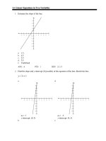
4. Which of the following is a sketch of the graph of the function y ϭ ͑x Ϫ 1͒3?
y

(a)

(b)

y

3

•

2
1

1
−2

x

−1

2

1

2

3

−1

−2

(c)

−2

y

(d)

y
2

2

1

1

−1

x

x
1

−3

2

−2

−1

1
−1
−2

(e) None of these
5. Find an equation for the line passing through the point ͑4, Ϫ1͒ and parallel to the line 2x Ϫ 3y ϭ 3.
(a) 2x Ϫ 3y ϭ 11
2

(d) y ϭ 3x Ϫ 1

(b) 2x Ϫ 3y ϭ Ϫ5

© Houghton Mifflin Company. All rights reserved.

x
−1

•
•
•

(c) 3x Ϫ 2y ϭ Ϫ5

(e) None of these

•

New! HM Testing (powered by Diploma™)
For the instructor, HM Testing is a robust test-generating system.

Features
• Comprehensive set of algorithmic test items

• Can produce chapter tests, cumulative tests, and final
exams

• Online testing
• Gradebook function

xvi

This resource contains worked-out solutions to all textbook exercises in electronic format. It is available in three
volumes: Volume I covers Chapters 1–6, Volume II covers
Chapters 7–11, and Volume III covers Chapters 11–15.
Instructor’s Resource Guide by Ann Rutledge Kraus
This resource contains an abundance of resources keyed
to the textbook by chapter and section, including chapter
summaries, teaching strategies, multiple versions of chapter tests, final exams, and gateway tests, and suggested
solutions to the Chapter Openers, Explorations, Section
Projects, and Technology features in the text in electronic
format.
Test Item File The Test Item File contains a sample
question for every algorithm in HM Testing in electronic
format.
HM Testing test generator
Digital textbook art
Textbook Appendices D–F, containing additional
presentations with exercises covering precalculus review,
rotation and the general second degree equation, and
complex numbers.
Downloadable graphing calculator programs

Enhanced! Instructional DVDs and Videos
These comprehensive DVD and video presentations complement the textbook topic
coverage and have a variety of uses, including supplementing an online or hybrid
course, giving students the opportunity to catch up if they miss a class, and providing
substantial course material for self-study and review.

Features
• Comprehensive topic coverage from Calculus I, II, and III
• Additional explanations of calculus concepts, sample
problems, and applications

Enhanced! Companion Textbook Website
The free Houghton Mifflin website at college.hmco.com/pic/larsoncalculusetf4e
contains an abundance of instructor and student resources.

Features
• Downloadable graphing calculator programs
• Textbook Appendices D – F, containing additional presentations with exercises
covering precalculus review, rotation and the general second-degree equation,
and complex numbers
• Algebra Review Summary
• Calculus Labs

• 3-D rotatable graphs

Printed Resources
For the convenience of students, the Study and Solutions Guides are available
as printed supplements, but are also available in electronic format.
Study and Solutions Guide by Bruce Edwards
This student resource contains detailed, worked-out solutions to all

odd-numbered textbook exercises. It is available in two volumes: Volume I
covers Chapters 1–10 and Volume II covers Chapters 11–15.

For additional information about the Larson, Hostetler, and Edwards
Calculus program, go to college.hmco.com/info/larsoncalculus.
xvii


Features
Chapter Openers
Each chapter opens with a real-life application of
the concepts presented in the chapter, illustrated by
a photograph. Open-ended and thought-provoking
questions about the application encourage the
student to consider how calculus concepts relate to
real-life situations. A brief summary with a graphical
component highlights the primary mathematical
concepts presented in the chapter, and explains why
they are important.

3

Differentiation

You pump air at a steady rate into a deflated balloon until the balloon
bursts. Does the diameter of the balloon change faster when you first
start pumping the air, or just before the balloon bursts? Why?

To approximate the slope of a
tangent line to a graph at a given

point, find the slope of the secant
line through the given point and a
second point on the graph. As the
second point approaches the given
point, the approximation tends to
become more accurate. In Section
3.1, you will use limits to find
slopes of tangent lines to graphs.
This process is called differentiation.
Dr. Gary Settles/SPL/Photo Researchers

116

CHAPTER 3

Differentiation

Section 3.1

The Derivative and the Tangent Line Problem

115

• Find the slope of the tangent line to a curve at a point.
• Use the limit definition to find the derivative of a function.
• Understand the relationship between differentiability and continuity.

■ Cyan ■ Magenta ■ Yellow ■ Black
TY1

AC

QC

TY2

FR

Larson Texts, Inc. • Final Pages for Calc ETF 4/e

LARSON

Short

Long

The Tangent Line Problem
Mary Evans Picture Library

Calculus grew out of four major problems that European mathematicians were working on during the seventeenth century.
1.
2.
3.
4.
ISAAC NEWTON (1642–1727)

In addition to his work in calculus, Newton
made revolutionary contributions to physics,
including the Law of Universal Gravitation
and his three laws of motion.

y

P

x

Section Openers

The tangent line problem (Section 2.1 and this section)
The velocity and acceleration problem (Sections 3.2 and 3.3)
The minimum and maximum problem (Section 4.1)
The area problem (Sections 2.1 and 5.2)

Each problem involves the notion of a limit, and calculus can be introduced with any
of the four problems.
A brief introduction to the tangent line problem is given in Section 2.1. Although
partial solutions to this problem were given by Pierre de Fermat (1601–1665), René
Descartes (1596–1650), Christian Huygens (1629–1695), and Isaac Barrow
(1630 –1677), credit for the first general solution is usually given to Isaac Newton
(1642–1727) and Gottfried Leibniz (1646–1716). Newton’s work on this problem
stemmed from his interest in optics and light refraction.
What does it mean to say that a line is tangent to a curve at a point? For a circle,
the tangent line at a point P is the line that is perpendicular to the radial line at point
P, as shown in Figure 3.1.
For a general curve, however, the problem is more difficult. For example, how
would you define the tangent lines shown in Figure 3.2? You might say that a line is
tangent to a curve at a point P if it touches, but does not cross, the curve at point P.
This definition would work for the first curve shown in Figure 3.2, but not for the
second. Or you might say that a line is tangent to a curve if the line touches or

intersects the curve at exactly one point. This definition would work for a circle but
not for more general curves, as the third curve in Figure 3.2 shows.
y

y

y

y = f (x)

Tangent line to a circle
Figure 3.1

P

P
P

x

y = f (x)

y = f (x)

x

Tangent line to a curve at a point
FOR FURTHER INFORMATION For
more information on the crediting of
mathematical discoveries to the first

“discoverer,” see the article
“Mathematical Firsts—Who Done It?”
by Richard H. Williams and Roy D.
Mazzagatti in Mathematics Teacher.
To view this article, go to the website
www.matharticles.com.

xviii

Figure 3.2

x

Every section begins with an outline of the key
concepts covered in the section. This serves as a
class planning resource for the instructor and
a study and review guide for the student.

Explorations
For selected topics, Explorations offer the opportunity
to discover calculus concepts before they are formally
introduced in the text, thus enhancing student understanding. This optional feature can be omitted at the
discretion of the instructor with no loss of continuity
in the coverage of the material.

E X P L O R AT I O N

Identifying a Tangent Line Use a graphing utility to graph the function
f ͑x͒ ϭ 2x 3 Ϫ 4x 2 ϩ 3x Ϫ 5. On the same screen, graph y ϭ x Ϫ 5, y ϭ 2x Ϫ 5,
and y ϭ 3x Ϫ 5. Which of these lines, if any, appears to be tangent to the graph

of f at the point ͑0, Ϫ5͒? Explain your reasoning.

Historical Notes
Integrated throughout the text, Historical Notes help
students grasp the basic mathematical foundations
of calculus.


FEATURES

xix

Theorems
SECTION 3.2

Basic Differentiation Rules and Rates of Change

133

All Theorems and Definitions are highlighted for
emphasis and easy reference. Proofs are shown for
selected theorems to enhance student understanding.

Derivatives of Exponential Functions

E X P L O R AT I O N

One of the most intriguing (and useful) characteristics of the natural exponential function is that it is its own derivative. Consider the following.

Use a graphing utility to graph the

function

Let f ͑x͒ ϭ e x.

e xϩ⌬x Ϫ e x
f ͑x͒ ϭ
⌬x
for ⌬x ϭ 0.01. What does this function represent? Compare this graph
with that of the exponential function.
What do you think the derivative of
the exponential function equals?

fЈ ͑x͒ ϭ lim

⌬x→0

f ͑x ϩ ⌬ x͒ Ϫ f ͑x͒
⌬x

e xϩ⌬x Ϫ e x
⌬x→0
⌬x
e x͑e ⌬x Ϫ 1͒
ϭ lim
⌬x→0
⌬x

Study Tip

ϭ lim

Located at point of use throughout the text, Study
Tips advise students on how to avoid common errors,
address special cases, and expand upon theoretical
concepts.

The definition of e
lim ͑1 ϩ ⌬ x͒1͞⌬x ϭ e

⌬x→0

tells you that for small values of ⌬ x, you have e Ϸ ͑1 ϩ ⌬ x͒1͞⌬x, which implies that
e ⌬x Ϸ 1 ϩ ⌬ x. Replacing e ⌬x by this approximation produces the following.
STUDY TIP The key to the formula for
the derivative of f ͑x͒ ϭ e x is the limit

lim ͑1 ϩ x͒

1͞x

x→0

e x ͓e ⌬x Ϫ 1͔
⌬x
e x ͓͑1 ϩ ⌬ x͒ Ϫ 1͔
ϭ lim
⌬x→0
⌬x
e x⌬ x
ϭ lim

⌬x→0 ⌬ x
ϭ ex

fЈ ͑x͒ ϭ lim

⌬x→0

ϭ e.

This important limit was introduced on
page 51 and formalized later on page 85.
It is used to conclude that for ⌬x Ϸ 0,

͑1 ϩ ⌬x͒1͞⌬ x Ϸ e.

Graphics

This result is stated in the next theorem.

THEOREM 3.7

Numerous graphics throughout the text enhance
student understanding of complex calculus concepts
(especially in three-dimensional representations), as
well as real-life applications.

Derivative of the Natural Exponential Function

d x
͓e ͔ ϭ e x

dx

y

At the point (1, e),
the slope is e ≈ 2.72.

4

Derivatives of Exponential Functions

3

EXAMPLE 9

2

Find the derivative of each function.
a. f ͑x͒ ϭ 3e x

f (x) = e x
At the point (0, 1),
the slope is 1.
1

b. f ͑x͒ ϭ x 2 ϩ e x

c. f ͑x͒ ϭ sin x Ϫ e x

Solution

x

−2

You can interpret Theorem 3.7 graphically by saying that the slope of the graph
of f ͑x͒ ϭ e x at any point ͑x, e x͒ is equal to the y-coordinate of the point, as shown in
Figure 3.20.

2

Figure 3.20

d x
͓e ͔ ϭ 3e x
dx
d 2
d
b. fЈ ͑x͒ ϭ ͓x ͔ ϩ ͓e x͔ ϭ 2x ϩ e x
dx
dx
d
d
c. fЈ ͑x͒ ϭ ͓sin x͔ Ϫ ͓e x͔ ϭ cos x Ϫ e x
dx
dx
a. fЈ ͑x͒ ϭ 3

168

CHAPTER 3

Example
To enhance the usefulness of the text as a study and
learning tool, the Fourth Edition contains numerous
Examples. The detailed, worked-out Solutions (many
with side comments to clarify the steps or the
method) are presented graphically, analytically, and/or
numerically to provide students with opportunities for
practice and further insight into calculus concepts.
Many Examples incorporate real-data analysis.

Differentiation

y

It is meaningless to solve for dy͞dx in an equation that has no solution points.
(For example, x 2 ϩ y 2 ϭ Ϫ4 has no solution points.) If, however, a segment of a
graph can be represented by a differentiable function, dy͞dx will have meaning as the
slope at each point on the segment. Recall that a function is not differentiable at (1)
points with vertical tangents and (2) points at which the function is not continuous.

1

x2

+

y2

=0

(0, 0)
x

−1

1

EXAMPLE 3

−1

a. x 2 ϩ y 2 ϭ 0

y

y=

1

1 − x2

(−1, 0)

a. The graph of this equation is a single point. So, the equation does not define y as
a differentiable function of x.
b. The graph of this equation is the unit circle, centered at ͑0, 0͒. The upper semicircle
is given by the differentiable function

x

1
−1

y=−

1 − x2

y ϭ Ί1 Ϫ x 2,

(b)

y=

y ϭ Ϫ Ί1 Ϫ x 2,

1−x

x

−1

y=−

x < 1

and the lower half of this parabola is given by the differentiable function

1−x

y ϭ Ϫ Ί1 Ϫ x,

(c)

Some graph segments can be represented by
differentiable functions.
Figure 3.28

x < 1.

At the point ͑1, 0͒, the slope of the graph is undefined.
EXAMPLE 4

Finding the Slope of a Graph Implicitly

Determine the slope of the tangent line to the graph of
x 2 ϩ 4y 2 ϭ 4
at the point ͑Ί2, Ϫ1͞Ί2 ͒. See Figure 3.29.

y

Solution

2

x 2 + 4y 2 = 4

x

−1

1

−2

Instructional Notes accompany many of the
Theorems, Definitions, and Examples to offer
additional insights or describe generalizations.

y ϭ Ί1 Ϫ x,

1

−1

Ϫ1 < x < 1.

At the points ͑Ϫ1, 0͒ and ͑1, 0͒, the slope of the graph is undefined.
c. The upper half of this parabola is given by the differentiable function

(1, 0)

Notes

Ϫ1 < x < 1

and the lower semicircle is given by the differentiable function

y

1

Eduspace® contains Open Explorations, which
investigate selected Examples using computer algebra
systems (Maple, Mathematica, Derive, and Mathcad).
The icon
identifies these Examples.

c. x ϩ y 2 ϭ 1

b. x 2 ϩ y 2 ϭ 1

Solution

(1, 0)

−1

Open Exploration

Representing a Graph by Differentiable Functions

If possible, represent y as a differentiable function of x (see Figure 3.28).

(a)

Figure 3.29

(

2, − 1
2

)

x 2 ϩ 4y 2 ϭ 4
dy
ϭ0
dx
dy Ϫ2x Ϫx
ϭ
ϭ
dx
8y
4y

2x ϩ 8y

Write original equation.
Differentiate with respect to x.
Solve for

dy
.
dx

So, at ͑Ί2, Ϫ1͞Ί2 ͒, the slope is
dy
Ϫ Ί2
1

ϭ
ϭ .
dx Ϫ4͞Ί2 2

Evaluate

1
dy
when x ϭ Ί2 and y ϭ Ϫ
.
dx
Ί2

NOTE To see the benefit of implicit differentiation, try doing Example 4 using the explicit
function y ϭ Ϫ 12Ί4 Ϫ x 2.


xx

FEATURES

Exercises

In Exercises 63–66, find k such that the line is tangent to the
graph of the function.

The core of every calculus text, Exercises provide
opportunities for exploration, practice, and comprehension. The Fourth Edition contains over 10,000
Section and Chapter Review Exercises, carefully
graded in each set from skill-building to challenging.

The extensive range of problem types includes
true/false, writing, conceptual, real-data modeling,
and graphical analysis.

y ϭ 4x Ϫ 9

64. f ͑x͒ ϭ k Ϫ x 2
65. f ͑x͒ ϭ

Putnam Exam Challenge

Line

Function
63. f ͑x͒ ϭ x 2 Ϫ kx

186. Let f ͑x͒ ϭ a1 sin x ϩ a2 sin 2x ϩ . . . ϩ an sin nx, where
a1, a2, . . ., an are real numbers and where n is a positive
integer. Given that Խ f ͑x͒Խ ≤ Խsin xԽ for all real x, prove that
Խa1 ϩ 2a2 ϩ . . . ϩ nanԽ ≤ 1.

y ϭ Ϫ4x ϩ 7

k
x

3
yϭϪ xϩ3
4

66. f ͑x͒ ϭ
y ϭ xatϩ which
4
In Exercises
81–kΊ
86,x describe the x-values
f is
differentiable.
81. f ͑x͒ ϭ

1
xϩ1

Pn͑x͒
͑x k Ϫ 1͒nϩ1

82. f ͑x͒ ϭ Խx 2 Ϫ 9Խ
y

y

where Pn͑x͒ is a polynomial. Find Pn͑1͒.

12
10
1

−1

1

−4

−2

83. f ͑x͒ ϭ ͑x Ϫ 3͒ 2͞3

These problems were composed by the Committee on the Putnam Prize Competition.
© The Mathematical Association of America. All rights reserved.

6
4
2

x
−2

1
187. Let k be a fixed positive integer. The nth derivative of k
x Ϫ1
has the form

−2

2

x
4 True

or False? In Exercises 183–185, determine whether the
statement is true or false. If it is false, explain why or give an

example that shows it is false.

−4

84. f ͑x͒ ϭ

x2
x2 Ϫ 4

y

183. If y ϭ ͑1 Ϫ x͒1ր2, then yЈ ϭ 12͑1 Ϫ x͒Ϫ1ր2.
184. If f ͑x͒ ϭ sin 2͑2x͒, then fЈ͑x͒ ϭ 2͑sin 2x͒͑cos 2x͒.

y

185. If y is a differentiable function of u, u is a differentiable
function of v, and v is a differentiable function of x, then

5
4
3
2

5
4
3

x

1

−4

x
1 2 3 4 5 6

3 4

dy du dv
dy
ϭ Modeling
. Data The table shows the temperature T (ЊF) at
167.
dx du dv dx
which water boils at selected pressures p (pounds per square
inch). (Source: Standard Handbook of Mechanical Engineers)

−3

Ά

p

5

10

14.696 (1 atm)

20

T

162.24Њ

193.21Њ

212.00Њ

227.96Њ

p

30

40

60

80

100

T

250.33Њ

267.25Њ

292.71Њ

312.03Њ

327.81Њ

A model that approximates the data is
T ϭ 87.97 ϩ 34.96 ln p ϩ 7.91Ίp.
P.S.

P.S.

Problem Solving

201

(a) Find the radius r of the largest possible circle centered on the
y-axis that is tangent to the parabola at the origin, as
indicated in the figure. This circle is called the circle of
curvature (see Section 12.5). Use a graphing utility to graph
the circle and parabola in the same viewing window.
(b) Find the center ͑0, b͒ of the circle of radius 1 centered on the
y-axis that is tangent to the parabola at two points, as
indicated in the figure. Use a graphing utility to graph the
circle and parabola in the same viewing window.
y

5. Find a third-degree polynomial p͑x͒ that is tangent to the line
y ϭ 14x Ϫ 13 at the point ͑1, 1͒, and tangent to the line
y ϭ Ϫ2x Ϫ 5 at the point ͑Ϫ1, Ϫ3͒.

6. Find a function of the form f ͑x͒ ϭ a ϩ b cos cx that is tangent
to the line y ϭ 1 at the point ͑0, 1͒, and tangent to the line
yϭxϩ

3 ␲
Ϫ
2
4

at the point

΂␲4 , 23΃.

7. The graph of the eight curve,

y

x 4 ϭ a2͑x 2 Ϫ y 2͒, a

0,

2

(0, b)
1

is shown below.
y

1

r
x

−1

1

Figure for 1(a)

x

−1

1

−a

3. (a) Find the polynomial P1͑x͒ ϭ a0 ϩ a1x whose value and
slope agree with the value and slope of f ͑x͒ ϭ cos x at the
point x ϭ 0.
(b) Find the polynomial P2͑x͒ ϭ a0 ϩ a1x ϩ a2 x 2 whose value
and first two derivatives agree with the value and first two
derivatives of f ͑x͒ ϭ cos x at the point x ϭ 0. This polynomial is called the second-degree Taylor polynomial of
f ͑x͒ ϭ cos x at x ϭ 0.
(c) Complete the table comparing the values of f and P2. What
do you observe?
Ϫ1.0

a

Ϫ0.1

Ϫ0.001

0

0.001

0.1

(a) Explain how you could use a graphing utility to obtain the
graph of this curve.
(b) Use a graphing utility to graph the curve for various values
of the constant a. Describe how a affects the shape of the
curve.
(c) Determine the points on the curve where the tangent line is
horizontal.
8. The graph of the pear-shaped quartic,
b2y 2 ϭ x3͑a Ϫ x͒, a, b > 0,
is shown below.
y

1.0

cos x

x

a

P2ͧxͨ
(d) Find the third-degree Taylor polynomial of f ͑x͒ ϭ sin x at
x ϭ 0.
4. (a) Find an equation of the tangent line to the parabola y ϭ x 2 at
the point ͑2, 4͒.

(a) Explain how you could use a graphing utility to obtain the
graph of this curve.

(b) Find an equation of the normal line to y ϭ x 2 at the point
͑2, 4͒. (The normal line is perpendicular to the tangent line.)
Where does this line intersect the parabola a second time?

(b) Use a graphing utility to graph the curve for various values
of the constants a and b. Describe how a and b affect the
shape of the curve.

(c) Find equations of the tangent line and normal line to y ϭ x
at the point ͑0, 0͒.

(c) Determine the points on the curve where the tangent line is
horizontal.

2

(d) Prove that for any point ͑a, b͒ ͑0, 0͒ on the parabola
y ϭ x 2, the normal line intersects the graph a second time.

P.S. Problem Solving

Each chapter concludes with a set of thoughtprovoking and challenging exercises that provide
opportunities for the student to explore the concepts
in the chapter further.

x

Figure for 1(b)

2. Graph the two parabolas y ϭ x 2 and y ϭ Ϫx 2 ϩ 2x Ϫ 5 in the
same coordinate plane. Find equations of the two lines simultaneously tangent to both parabolas.

x

(b) Find the rate of change of T with respect to p when
p ϭ 10 and p ϭ 70.

See www.CalcChat.com for worked-out solutions to odd-numbered exercises.

1. Consider the graph of the parabola y ϭ x 2.

2

Problem Solving

(a) Use a graphing utility to plot the data and graph the
model.

Technology
Throughout the text, the use of a graphing utility or
computer algebra system is suggested as appropriate

for problem-solving as well as exploration and
discovery. For example, students may choose to
use a graphing utility to execute complicated
computations, to visualize theoretical concepts, to
discover alternative approaches, or to verify the
results of other solution methods. However, students
are not required to have access to a graphing utility
to use this text effectively. In addition to describing
the benefits of using technology to learn calculus,
the text also addresses its possible misuse or
misinterpretation.

Additional Features
Additional teaching and learning resources are integrated throughout the
textbook, including Section Projects, journal references, and Writing About
Concepts Exercises.


Acknowledgments
We would like to thank the many people who have helped us at various stages of this
project over the years. Their encouragement, criticisms, and suggestions have been
invaluable to us.

For the Fourth Edition
Andre Adler
Illinois Institute of Technology

Angela Hare
Messiah College

Evelyn Bailey
Oxford College of Emory University

Karl Havlak
Angelo State University

Katherine Barringer
Central Virginia Community College

James Herman
Cecil Community College

Robert Bass
Gardner-Webb University

Xuezhang Hou
Towson University

Joy Becker
University of Wisconsin Stout

Gene Majors
Fullerton College

Michael Bezusko
Pima Community College

Suzanne Molnar
College of St. Catherine

Bob Bradshaw
Ohlone College

Karen Murany
Oakland Community College

Robert Brown
The Community College of Baltimore
County (Essex Campus)

Keith Nabb
Moraine Valley Community College

Joanne Brunner
DePaul University
Minh Bui
Fullerton College
Fang Chen
Oxford College of Emory University
Alex Clark
University of North Texas
Jeff Dodd
Jacksonville State University
Daniel Drucker
Wayne State University

Stephen Nicoloff
Paradise Valley Community College
James Pommersheim
Reed College

James Ralston
Hawkeye Community College
Chip Rupnow
Martin Luther College
Mark Snavely
Carthage College
Ben Zandy
Fullerton College

Pablo Echeverria
Camden County College

xxi


xxii

ACKNOWLEDGMENTS

For the Fourth Edition Technology Program
Jim Ball
Indiana State University

Arek Goetz
San Francisco State University

Marcelle Bessman
Jacksonville University

John Gosselin

University of Georgia

Tim Chappell
Penn Valley Community College

Shahryar Heydari
Piedmont College

Oiyin Pauline Chow
Harrisburg Area Community College

Douglas B. Meade
University of South Carolina

Julie M. Clark
Hollins University

Teri Murphy
University of Oklahoma

Jim Dotzler
Nassau Community College

Howard Speier
Chandler-Gilbert Community College

Murray Eisenberg
University of Massachusetts at Amherst

Reviewers of Previous Editions

Raymond Badalian
Los Angeles City College

Kathy Hoke
University of Richmond

Norman A. Beirnes
University of Regina

Howard E. Holcomb
Monroe Community College

Christopher Butler
Case Western Reserve University

Gus Huige
University of New Brunswick

Dane R. Camp
New Trier High School, IL

E. Sharon Jones
Towson State University

Jon Chollet
Towson State University

Robert Kowalczyk
University of Massachusetts–Dartmouth

Barbara Cortzen
DePaul University

Anne F. Landry
Dutchess Community College

Patricia Dalton
Montgomery College

Robert F. Lax
Louisiana State University

Luz M. DeAlba
Drake University

Beth Long
Pellissippi State Technical College

Dewey Furness
Ricks College

Gordon Melrose
Old Dominion University

Javier Garza
Tarleton State University

Bryan Moran
Radford University

Claire Gates
Vanier College

David C. Morency
University of Vermont

Lionel Geller
Dawson College

Guntram Mueller
University of Massachusetts–Lowell

Carollyne Guidera
University College of Fraser Valley

Donna E. Nordstrom
Pasadena City College

Irvin Roy Hentzel
Iowa State University

Larry Norris
North Carolina State University


ACKNOWLEDGMENTS

xxiii

Mikhail Ostrovskii

Catholic University of America

Lynn Smith
Gloucester County College

Jim Paige
Wayne State College

Linda Sundbye
Metropolitan State College of Denver

Eleanor Palais
Belmont High School, MA

Anthony Thomas
University of Wisconsin–Platteville

James V. Rauff
Millikin University

Robert J. Vojack
Ridgewood High School, NJ

Lila Roberts
Georgia Southern University

Michael B. Ward
Bucknell University

David Salusbury

John Abbott College

Charles Wheeler
Montgomery College

John Santomas
Villanova University
During the past four years, several users of the Third Edition wrote to us with
suggestions. We considered each and every one of them when preparing the manuscript
for the Fourth Edition. A special note of thanks goes to the instructors and to the
students who have used earlier editions of the text.
We would like to thank the staff at Larson Texts, Inc., who assisted with
proofreading the manuscript, preparing and proofreading the art package, and checking
and typesetting the supplements.
On a personal level, we are grateful to our wives, Deanna Gilbert Larson, Eloise
Hostetler, and Consuelo Edwards, for their love, patience, and support. Also, a special
note of thanks goes to R. Scott O’Neil.
If you have suggestions for improving this text, please feel free to write to us. Over
the years we have received many useful comments from both instructors and students,
and we value these very much.
Ron Larson

Robert Hostetler

Bruce H. Edwards


This page intentionally left blank