Introduction to singularities and deformations
Bạn đang xem bản rút gọn của tài liệu. Xem và tải ngay bản đầy đủ của tài liệu tại đây (4.27 MB, 481 trang )
Springer Monographs in Mathematics
G.-M. Greuel • C. Lossen • E. Shustin
Introduction to
Singularities and
Deformations
www.pdfgrip.com
Gert-Martin Greuel
Fachbereich Mathematik
Universität Kaiserslautern
Erwin-Schrödinger-Str.
67663 Kaiserslautern, Germany
e-mail:
Christoph Lossen
Fachbereich Mathematik
Universität Kaiserslautern
Erwin-Schrödinger-Str.
67663 Kaiserslautern, Germany
e-mail:
Eugenii Shustin
School of Mathematical Sciences
Raymond and Beverly Sackler Faculty of Exact Sciences
Tel Aviv University
Ramat Aviv
69978 Tel Aviv, Israel
e-mail:
Library of Congress Control Number: 2006935374
Mathematics Subject Classification (2000): 14B05, 14B07, 14B10, 14B12, 14B25, 14Dxx,
14H15, 14H20, 14H50, 13Hxx, 14Qxx
ISSN 1439-7382
ISBN-10 3-540-28380-3 Springer Berlin Heidelberg New York
ISBN-13 978-3-540-28380-5 Springer Berlin Heidelberg New York
This work is subject to copyright. All rights are reserved, whether the whole or part of the material is concerned, specifically
the rights of translation, reprinting, reuse of illustrations, recitation, broadcasting, reproduction on microfilm or in any other
way, and storage in data banks. Duplication of this publication or parts thereof is permitted only under the provisions of the
German Copyright Law of September 9, 1965, in its current version, and permission for use must always be obtained from
Springer. Violations are liable for prosecution under the German Copyright Law.
Springer is a part of Springer Science+Business Media
springer.com
c Springer-Verlag Berlin Heidelberg 2007
The use of general descriptive names, registered names, trademarks, etc. in this publication does not imply, even in the
absence of a specific statement, that such names are exempt from the relevant protective laws and regulations and therefore
free for general use.
Typesetting by the authors and VTEX using a Springer LATEX macro package
Cover design: Erich Kirchner, Heidelberg, Germany
Printed on acid-free paper
SPIN: 10820313
VA 4141/3100/VTEX - 5 4 3 2 1 0
www.pdfgrip.com
Meiner Mutter Irma und
der Erinnerung meines Vaters Wilhelm
G.-M.G.
Fă
ur Carmen, Katrin und Carolin
C.L.
To my parents Isaac and Maya
E.S.
www.pdfgrip.com
VI
A deformation of a simple surface singularity of type E7 into four A1 singularities. The family is defined by the equation
F (x, y, z; t) = z 2 −
x+
4t3
27
· x2 − y 2 (y + t) .
The pictures1 show the surface obtained for t = 0, t = 14 , t =
1
1
2
and t = 1.
The pictures were drawn by using the program surf which is distributed with
Singular [GPS].
www.pdfgrip.com
Preface
Singularity theory is a field of intensive study in modern mathematics with
fascinating relations to algebraic geometry, complex analysis, commutative
algebra, representation theory, the theory of Lie groups, topology, dynamical
systems, and many more, and with numerous applications in the natural and
technical sciences. The specific feature of the present Introduction to Singularities and Deformations, separating it from other introductions to singularity
theory, is the choice of a material and a unified point of view based on the
theory of analytic spaces.
This text has grown up from a preparatory part of our monograph Singular algebraic curves (to appear), devoted to the up-to-date theory of equisingular families of algebraic curves and related topics such as local and global
deformation theory, the cohomology vanishing theory for ideal sheaves of zerodimensional schemes associated with singularities, applications and computational aspects. When working at the monograph, we realized that in order to
keep the required level of completeness, accuracy, and readability, we have to
provide a relevant and exhaustive introduction. Indeed, many needed statements and definitions have been spread through numerous sources, sometimes
presented in a too short or incomplete form, and often in a rather different
setting. This, finally, has led us to the decision to write a separate volume,
presenting a self-contained textbook on the basic singularity theory of analytic spaces, including local deformation theory, and the theory of plane curve
singularities.
Having in mind to get the reader ready for understanding the volume
Singular algebraic curves, we did not restrict the book to that specific purpose.
The present book comprises material which can partly be found in other books
and partly in research articles, and which for the first time is exposed from
a unified point of view, with complete proofs which are new in many cases.
We include many examples and exercises which complement and illustrate
the general theory. This exposition can serve as a source for special courses
in singularity theory and local algebraic and analytic geometry. A special
attention is paid to the computational aspect of the theory, illustrated by a
www.pdfgrip.com
VIII
Preface
number of examples of computing various characteristics via the computer
algebra system Singular [GPS]2 . Three appendices, including basic facts
from sheaf theory, commutative algebra, and formal deformation theory, make
the reading self-contained.
In the first part of the book we develop the relevant techniques, the basic theory of complex spaces and their germs and sheaves on them, including
the key ingredients - the Weierstraß preparation theorem and its other forms
(division theorem and finiteness theorem), and the finite coherence theorem.
Then we pass to the main object of study, isolated hypersurface and plane
curve singularities. Isolated hypersurface singularities and especially plane
curve singularities form a classical research area which still is in the centre of
current research. In many aspects they are simpler than general singularities,
but on the other hand they are much richer in ideas, applications, and links
to other branches of mathematics. Furthermore, they provide an ideal introduction to the general singularity theory. Particularly, we treat in detail the
classical topological and analytic invariants, finite determinacy, resolution of
singularities, and classification of simple singularities.
In the second chapter, we systematically present the local deformation
theory of complex space germs with an emphasis on the issues of versality,
infinitesimal deformations and obstructions. The chapter culminates in the
treatment of equisingular deformations of plane curve singularities. This is a
new treatment, based on the theory of deformations of the parametrization
developed here with a complete treatment of infinitesimal deformations and
obstructions for several related functors. We further provide a full disquisition on equinormalizable (δ-constant) deformations and prove that after base
change, by normalizing the δ-constant stratum, we obtain the semiuniversal
deformation of the parametrization. Equisingularity is first introduced for deformations of the parametrization and it is shown that this is essentially a
linear theory and, thus, the corresponding semiuniversal deformation has a
smooth base. By proving that the functor of equisingular deformations of the
parametrization is isomorphic to the functor of equisingular deformations of
the equation, we substantially enhance the original work by J. Wahl [Wah],
and, in particular, give a new proof of the smoothness of the μ-constant stratum. Actually, this part of the book is intended for a more advanced reader
familiar with the basics of modern algebraic geometry and commutative algebra. A number of illustrating examples and exercises should make the material
more accessible and keep the textbook style, suitable for special courses on
the subject.
Cross references to theorems, propositions, etc., within the same chapter are
given by, e.g., “Theorem 1.1”. References to statements in another chapter
are preceded by the chapter number, e.g., “Theorem I.1.1”.
2
See [GrP, DeL] for a thorough introduction to Singular and its applicability to
problems in algebraic geometry and singularity theory.
www.pdfgrip.com
Preface
IX
Acknowledgements
Our work at the monograph has been supported by the Herman Minkowsky–
Minerva Center for Geometry at Tel–Aviv University, by grant no. G-61615.6/99 from the German-Israeli Foundation for Research and Development
and by the Schwerpunkt “Globale Methoden in der komplexen Geometrie”
of the Deutsche Forschungsgemeinschaft. We have significantly advanced in
our project during our two ”Research-in-Pairs” stays at the Mathematisches
Forschungsinstitut Oberwolfach. E. Shustin was also supported by the Bessel
Research Award from the Alexander von Humboldt Foundation.
Our communication with Antonio Campillo, Steve Kleiman and Jonathan
Wahl was invaluable for successfully completing our work. We also are very
grateful to Thomas Markwig, Ilya Tyomkin and Eric Westenberger for proofreading and for partly typing the manuscript.
Kaiserslautern - Tel Aviv,
August 2006
G.-M. Greuel, C. Lossen,
and E. Shustin
www.pdfgrip.com
X
Preface
(a)
(b)
Deformations of a simple surface singularity of type E7 (a) into two A1 singularities and one A3 -singularity, resp. (b) into two A1 -singularities,
smoothing the A3 -singularity. The corresponding family is defined by
F (x, y, z; t) = z 2 − x +
3√3
t
10
· x2 − y 2 (y + t) ,
F (x, y, z; t) = z 2 − x +
6√3
t
10
· x2 − y 2 (y + t) .
resp. by
www.pdfgrip.com
Contents
Chapter I
Singularity Theory . . . . . . . . . . . . . . . . . . . . . . . . . . . . . . 1
1 Basic Properties of Complex Spaces and Germs . . . . . . . . . . . . . . . 8
1.1 Weierstraß Preparation and Finiteness Theorem . . . . . . . . . 8
1.2 Application to Analytic Algebras . . . . . . . . . . . . . . . . . . . . . . 23
1.3 Complex Spaces . . . . . . . . . . . . . . . . . . . . . . . . . . . . . . . . . . . . . 35
1.4 Complex Space Germs and Singularities . . . . . . . . . . . . . . . . 55
1.5 Finite Morphisms and Finite Coherence Theorem . . . . . . . . 64
1.6 Applications of the Finite Coherence Theorem . . . . . . . . . . . 75
1.7 Finite Morphisms and Flatness . . . . . . . . . . . . . . . . . . . . . . . . 80
1.8 Flat Morphisms and Fibres . . . . . . . . . . . . . . . . . . . . . . . . . . . 87
1.9 Normalization and Non-Normal Locus . . . . . . . . . . . . . . . . . . 94
1.10 Singular Locus and Differential Forms . . . . . . . . . . . . . . . . . . 100
2 Hypersurface Singularities . . . . . . . . . . . . . . . . . . . . . . . . . . . . . . . . . 110
2.1 Invariants of Hypersurface Singularities . . . . . . . . . . . . . . . . . 110
2.2 Finite Determinacy . . . . . . . . . . . . . . . . . . . . . . . . . . . . . . . . . . 126
2.3 Algebraic Group Actions . . . . . . . . . . . . . . . . . . . . . . . . . . . . . . 135
2.4 Classification of Simple Singularities . . . . . . . . . . . . . . . . . . . . 144
3 Plane Curve Singularities . . . . . . . . . . . . . . . . . . . . . . . . . . . . . . . . . . 161
3.1 Parametrization . . . . . . . . . . . . . . . . . . . . . . . . . . . . . . . . . . . . . 162
3.2 Intersection Multiplicity . . . . . . . . . . . . . . . . . . . . . . . . . . . . . . 174
3.3 Resolution of Plane Curve Singularities . . . . . . . . . . . . . . . . . 181
3.4 Classical Topological and Analytic Invariants . . . . . . . . . . . . 201
Chapter II. Local Deformation Theory . . . . . . . . . . . . . . . . . . . . . . . 221
1 Deformations of Complex Space Germs . . . . . . . . . . . . . . . . . . . . . . 222
1.1 Deformations of Singularities . . . . . . . . . . . . . . . . . . . . . . . . . . 222
1.2 Embedded Deformations . . . . . . . . . . . . . . . . . . . . . . . . . . . . . . 228
1.3 Versal Deformations . . . . . . . . . . . . . . . . . . . . . . . . . . . . . . . . . . 234
1.4 Infinitesimal Deformations . . . . . . . . . . . . . . . . . . . . . . . . . . . . 246
1.5 Obstructions . . . . . . . . . . . . . . . . . . . . . . . . . . . . . . . . . . . . . . . . 259
2 Equisingular Deformations of Plane Curve Singularities . . . . . . . . 266
www.pdfgrip.com
XII
Contents
2.1
2.2
2.3
2.4
2.5
2.6
2.7
2.8
Equisingular Deformations of the Equation . . . . . . . . . . . . . . 267
The Equisingularity Ideal . . . . . . . . . . . . . . . . . . . . . . . . . . . . . 282
Deformations of the Parametrization . . . . . . . . . . . . . . . . . . . 296
Computation of T 1 and T 2 . . . . . . . . . . . . . . . . . . . . . . . . . . . . 308
Equisingular Deformations of the Parametrization . . . . . . . . 322
Equinormalizable Deformations . . . . . . . . . . . . . . . . . . . . . . . . 340
δ-Constant and μ-Constant Stratum . . . . . . . . . . . . . . . . . . . . 352
Comparison of Equisingular Deformations . . . . . . . . . . . . . . . 360
Appendix A. Sheaves . . . . . . . . . . . . . . . . . . . . . . . . . . . . . . . . . . . . . . . . . . 379
A.1 Presheaves and Sheaves . . . . . . . . . . . . . . . . . . . . . . . . . . . . . . . . . . . . 379
A.2 Gluing Sheaves . . . . . . . . . . . . . . . . . . . . . . . . . . . . . . . . . . . . . . . . . . . 381
A.3 Sheaves of Rings and Modules . . . . . . . . . . . . . . . . . . . . . . . . . . . . . . 382
A.4 Image and Preimage Sheaf . . . . . . . . . . . . . . . . . . . . . . . . . . . . . . . . . 383
A.5 Algebraic Operations on Sheaves . . . . . . . . . . . . . . . . . . . . . . . . . . . . 384
A.6 Ringed Spaces . . . . . . . . . . . . . . . . . . . . . . . . . . . . . . . . . . . . . . . . . . . . 385
A.7 Coherent Sheaves . . . . . . . . . . . . . . . . . . . . . . . . . . . . . . . . . . . . . . . . . 387
A.8 Sheaf Cohomology . . . . . . . . . . . . . . . . . . . . . . . . . . . . . . . . . . . . . . . . 388
ˇ
A.9 Cech
Cohomology and Comparison . . . . . . . . . . . . . . . . . . . . . . . . . . 392
Appendix B. Commutative Algebra . . . . . . . . . . . . . . . . . . . . . . . . . . . 397
B.1 Associated Primes and Primary Decomposition . . . . . . . . . . . . . . . 397
B.2 Dimension Theory . . . . . . . . . . . . . . . . . . . . . . . . . . . . . . . . . . . . . . . . 399
B.3 Tensor Product and Flatness . . . . . . . . . . . . . . . . . . . . . . . . . . . . . . . 402
B.4 Artin-Rees and Krull Intersection Theorem . . . . . . . . . . . . . . . . . . 406
B.5 The Local Criterion of Flatness . . . . . . . . . . . . . . . . . . . . . . . . . . . . . 407
B.6 The Koszul Complex . . . . . . . . . . . . . . . . . . . . . . . . . . . . . . . . . . . . . . 410
B.7 Regular Sequences and Depth . . . . . . . . . . . . . . . . . . . . . . . . . . . . . . 414
B.8 Cohen-Macaulay, Flatness and Fibres . . . . . . . . . . . . . . . . . . . . . . . . 416
B.9 Auslander-Buchsbaum Formula . . . . . . . . . . . . . . . . . . . . . . . . . . . . . 422
Appendix C. Formal Deformation Theory . . . . . . . . . . . . . . . . . . . . . 425
C.1 Functors of Artin Rings . . . . . . . . . . . . . . . . . . . . . . . . . . . . . . . . . . . . 425
C.2 Obstructions . . . . . . . . . . . . . . . . . . . . . . . . . . . . . . . . . . . . . . . . . . . . . 431
C.3 The Cotangent Complex . . . . . . . . . . . . . . . . . . . . . . . . . . . . . . . . . . . 436
C.4 Cotangent Cohomology . . . . . . . . . . . . . . . . . . . . . . . . . . . . . . . . . . . . 441
C.5 Relation to Deformation Theory . . . . . . . . . . . . . . . . . . . . . . . . . . . . 443
References . . . . . . . . . . . . . . . . . . . . . . . . . . . . . . . . . . . . . . . . . . . . . . . . . . . . . 447
Index . . . . . . . . . . . . . . . . . . . . . . . . . . . . . . . . . . . . . . . . . . . . . . . . . . . . . . . . . . 455
www.pdfgrip.com
I
Singularity Theory
“The theory of singularities of differentiable maps is a rapidly developing area of contemporary mathematics, being a grandiose generalization of the study of functions at maxima and minima, and having
numerous applications in mathematics, the natural sciences and technology (as in the so-called theory of bifurcations and catastrophes).”
V.I. Arnol’d, S.M. Guzein-Zade, A.N. Varchenko [AGV].
The above citation describes in a few words the essence of what is called today often “singularity theory”. A little bit more precisely, we can say that
the subject of this relatively new area of mathematics is the study of systems of finitely many differentiable, or analytic, or algebraic, functions in the
neighbourhood of a point where the Jacobian matrix of these functions is not
of locally constant rank. The general notion of a “singularity” is, of course,
much more comprehensive. Singularities appear in all parts of mathematics,
for instance as zeroes of vector fields, or points at infinity, or points of indeterminacy of functions, but always refer to a situation which is not regular,
that is, not the usual, or expected, one.
In the first part of this book, we are mainly studying the singularities of
systems of complex analytic equations,
f1 (x1 , . . . , xn ) = 0 ,
..
..
.
.
fm (x1 , . . . , xn ) = 0 ,
(0.0.1)
where the fi are holomorphic functions in some open set of Cn . More precisely,
we investigate geometric properties of the solution set V = V (f1 , . . . , fm ) of
a system (0.0.1) in a small neighbourhood of those points, where the analytic
set V fails to be a complex manifold. In algebraic terms, this means to study
analytic C-algebras, that is, factor algebras of power series algebras over the
field of complex numbers. Both points of view, the geometric one and the
algebraic one, contribute to each other. Generally speaking, we can say that
geometry provides intuition, while algebra provides rigour.
www.pdfgrip.com
2
I Singularity Theory
Of course, the solution set of the system (0.0.1) in a small neighbourhood
of some point p = (p1 , . . . , pn ) ∈ Cn depends only on the ideal I generated by
f1 , . . . , fm in C{x − p} = C{x1 − p1 , . . . , xn − pn }. Even more, if J denotes the
uckert Nullstelideal generated by g1 , . . . , g in C{x − p}, then the Hilbert-Ră
,
.
.
.
,
f
)
=
V
(g
,
.
.
.
,
g
)
in
a
small
neighbourhood
of
lensatz
states
that
V
(f
1
m
1
p i I = J. Here, I := f ∈ C{x − p} f r ∈ I for some r ≥ 0 denotes
the radical of I.
Of course, this is analogous to Hilbert’s Nullstellensatz for solution sets
in Cn of complex polynomial equations and for ideals in the polynomial ring
C[x] = C[x1 , . . . , xn ]. The Nullstellensatz provides a bridge between algebra
and geometry.
The somewhat vague formulation “a sufficiently small neighbourhood of p
in V ” is made precise by the concept of the germ (V, p) of the analytic set V
at p. Then the Hilbert-Ră
uckert Nullstellensatz can be reformulated by saying
that two analytic functions, defined in some neighbourhood of p in √
Cn , define
the same function on the germ (V, p) iff their difference belongs to I. Thus,
the algebra√of complex analytic functions on the germ (V, p) is identified with
C{x − p}/ I.
√
However, although I and √I have the same solution set, we loose information when passing from I to I. This is similar to the univariate case, where
the sets V (x) and V (xk ) coincide, but where the zero of the polynomial x,
respectively xk , is counted with multiplicity 1, respectively with multiplicity
k. The significance of the multiplicity becomes immediately clear if we slightly
“deform” x, resp. xk : while x − t has only one root, (x − t)k has k different
roots for small t = 0. The notion of a complex space germ generalizes the
notion of a germ of an analytic set by taking into account these multiplicities. Formally, it is just a pair, consisting of the germ (V, p) and the algebra
C{x − p}/I. As (V, p) is determined by I, analytic C-algebras and germs of
complex spaces essentially carry the same information (the respective categories are equivalent). One is the algebraic, respectively the geometric, mirror
of the other. In this book, the word “singularity” will be used as a synonym
for “complex space germ”.
The concept of coherent analytic sheaves is used to pass from the local notion of a complex space germ to the global notion of a complex space. Indeed,
the theory of sheaves is unavoidable in modern algebraic and analytic geometry as a powerful tool for handling questions that involve local solutions and
global patching. Coherence of a sheaf can be understood as a local principle
of analytic continuation, which allows to pass from properties at a point p to
properties in a neighbourhood of p.
For easy reference, we give a short account of sheaf theory in Appendix
A. It should provide sufficient background on abstract sheaf theory for the
unexperienced reader. Anyway, it is better to learn about sheaves via concrete
examples such as the sheaf of holomorphic functions, than to start with the
rather abstract theory.
www.pdfgrip.com
I Singularity Theory
3
Section 1 gives an introduction to the theory of analytic C-algebras (even
of analytic K-algebras, where K is any complete real valued field), and to
complex spaces and germs of complex spaces. We develop the local Weierstraß
theory, which is fundamental to local analytic geometry. The central aim of
the first section is then to prove the finite coherence theorem, which states
that for a finite morphism f : X → Y of complex spaces, the direct image f∗ F
of a coherent OX -sheaf F is a coherent OY -sheaf.
The usefulness of the finite coherence theorem for singularity theory can
hardly be overestimated. Once it is proved, it provides a general, uniform
and powerful tool to prove theorems which otherwise are hard to obtain, even
in special cases. We use it, in particular, to prove the Hilbert-Ră
uckert Nullstellensatz, which provides the link between analytic geometry and algebra
indicated above. Moreover, the finite coherence theorem is used to give an
easy proof for the (semi)continuity of certain fibre functions.
This pays off in Section 2, where we study the solution set of only one
equation (m = 1 in (0.0.1)). The corresponding singularities, or the defining
power series, are called hypersurface singularities. Historically, hypersurface
singularities given by one equation in two variables, that is, plane curve singularities, can be seen as the initial point of singularity theory. For instance, in
Newton’s work on affine cubic plane curves, the following singularities appear:
{x2 − y 2 = 0}
{x2 − y 3 = 0}
{x2 y− y 2 = 0}
{x3 − xy 2 = 0}
The pictures only show the set of real solutions. However, in the given cases,
they also reflect the main geometric properties of the complex solution set in
a small neighbourhood of the origin, such as the number of irreducible components (corresponding to the irreducible factors of the defining polynomial
in the power series ring) and the pairwise intersection behaviour (transversal
or tangential) of these components.
In concrete examples, as above, singularities are given by polynomial equations. However, for a hypersurface singularity given by a polynomial, the
irreducible components do not necessarily have polynomial equations, too.
Consider, for instance, the plane cubic curve {x2 − y 2 (1 + y) = 0}:
{x2 − y 2 (1 + y) = 0}
www.pdfgrip.com
4
I Singularity Theory
While f := x2 − y 2 (1 + y) is irreducible in the polynomial ring C[x, y] (and in
its localization at x, y ), in the power series ring C{x, y} we have a decomposition
f = x−y 1+y x+y 1+y
√
√
into two non-trivial factors x ± y 1 + y ∈ C{x, y}. (Note that 1 + y is a unit
in C{x, y} but it is not an element of C[x, y].) As suggested by the picture,
this shows that in a small neighbourhood of the origin the curve has two
components, intersecting transversally, while in a bigger neighbourhood it is
irreducible.
From a geometric point of view, there is no difference between the singularities at the origin of {x2 − y 2 = 0} and of {f = 0}. Algebraically, this is
2
2
reflected by the fact that the factor
√ rings C{x, y}/ x − y and C{x, y}/ f
are isomorphic (via x → x, y → y 1 + y). We say that the two singularities
have the same analytic type, or that the defining equations are contact equivalent, if their factor algebras are isomorphic.
Closely related to contact equivalence is the notion of right equivalence:
two power series f and g are right equivalent if they coincide up to an analytic
change of coordinates. In the late 1960’s, V.I. Arnol’d started the classification of hypersurface singularities with respect to right equivalence. His work
culminated, among others, in impressive lists of normal forms of singularities [AGV, II.16]. The singularities in these lists turned out to be of great
improtance in other parts of mathematics and physics.
Most prominent is the list of simple, or Kleinian, or ADE-singularities,
which have appeared in surprisingly diverse areas of mathematics. The above
examples of plane curve singularities belong to this list: the corresponding
classes are named A1 , A2 , A3 and D4 . The letters A, D result from their
relation to the simple Lie groups of type A, D. The indices 1, . . . , 4 refer
to an important invariant of hypersurface singularities, the Milnor number,
which for simple singularities coincides with another important invariant, the
Tjurina number.
These invariants are introduced and studied in Section 2.1. We show, as an
application of the finite coherence theorem, that they behave semicontinuously
under deformation. Section 2.2 shows also that each isolated hypersurface
singularity f has a polynomial normal form. They are actually determined (up
to right as well as up to contact equivalence) by the Taylor series expansion
up to a sufficiently high order. The remaining part of Section 2 is devoted
to the (analytic) classification of singularities. In particular, in Section 2.4,
we give a full proof for the classification of simple singularities as given by
Arnol’d.
We actually do this for right and for contact equivalence. While the theory
with respect to right equivalence is well-developed, even in textbooks, this is
not the case for contact equivalence (which is needed in the second volume). It
appears that Section 2 provides the first systematic treatment with full proofs
for contact equivalence.
www.pdfgrip.com
I Singularity Theory
5
In Section 3, we focus on plane curve singularities, a particular case of hypersurface singularities, which is a classical object of study, but still in the
centre of current research. Plane curve singularities admit a much more deep
and complete description than general hypersurface singularities.
The aim of Section 3 is to present the two most powerful technical tools
— the parametrization of local branches (irreducible components of germs of
analytic curves) and the embedded resolution of singularities by a sequence
of blowing ups — and then to give the complete topological classification
of plane curve singularities. We also present a detailed treatment of various
topological and analytic invariants.
The existence of analytic parametrizations is naturally linked with
the algebraic closeness of the field of complex convergent Puiseux series
1/m
}, and it can be proved by Newton’s constructive method. Solvm≥1 C{x
ing a polynomial equation in two variables with respect to one of them, Newton introduced what is nowadays called a Newton diagram. Newton’s algorithm is a beautiful example of a combinatoric-geometric idea, solving an
algebraic-analytic problem.
An immediate application of parametrizations is realized in the study of
the intersection multiplicity of two plane curve germs, introduced as the total
order of one curve on the parametrizations of the local branches of the other
curve. This way of introducing the intersection multiplicity is quite convenient
in computations as well as in deriving the main properties of the intersection
multiplicity.
One of the most important geometric characterizations of plane curve singularities is based on the embedded resolution (desingularization) via subsequent blowing ups. Induction on the number of blowing ups to resolve the
singularity serves as a universal technical tool for proving various properties
and for computing numerical characteristics of plane curve singularities.
Our next goal is the topological classification of plane curve singularities.
In contrast to analytic or contact equivalence, the topological one does not
come from an algebraic group action. Another important distinction is that
the topological classification is discrete, that is, it has no moduli, whereas the
contact and right equivalences have. We give two descriptions of the topological type of a plane curve singularity: one via the characteristic exponents
of the Puiseux parametrizations of the local branches and their mutual intersection multiplicities, and another one via the sequence of infinitely near
points in the minimal embedded resolution and their multiplicities. Both descriptions are used to express the main topological numerical invariants, the
Milnor number (the maximal number of critical points in a small deformation
of the defining holomorphic function), the δ-invariant (the maximal number
of critical points lying on the deformed curve in a small deformation of the
curve germ), the κ-invariant (the number of ramification points of a generic
projection onto a line of a generic deformation), and the relations between
them.
www.pdfgrip.com
6
I Singularity Theory
General Notations and Conventions
We set N := {n ∈ Z | n ≥ 0}, the set of non-negative integers.
(A) Rings and Modules. We assume the reader to be familiar with the basic
facts from ideal and module theory. For more advanced topics, we refer to
Appendix B and the literature given there.
All rings A are assumed to be commutative with unit 1, all modules M are
unitary, that is, the multiplication by 1 is the identity map. If S is a subset
of A (resp. of M ), we denote by
S := S
A
ai fi | ai ∈ A, fi ∈ S
:=
finite
the ideal in A (resp. the submodule of M ) generated by S.
We say that M is a finite A-module or finite over A if M is generated as
A-module by a finite set. If ϕ : A → B is a ring map, I ⊂ A an ideal, and M
a B-module, then M is via am := ϕ(a)m an A-module and IM denotes the
submodule ϕ(I)M .
If K is a field, K[ε] denotes the two-dimensional K-algebra with ε2 = 0,
that is, K[ε] ∼
= K[x]/ x2 . If A is a local ring, mA or m denotes its maximal
ideal.
(B) Power Series and Polynomials. If α = (α1 , . . . , αn ) ∈ Nn , we use the
αn
1
standard notations xα = xα
1 · . . . · xn to denote monomials, and
∞
∞
cα xα =
f=
|α|=0
∞
αn
1
cα1 ···αn xα
1 · . . . · xn ,
cα xα =
α∈Nn
α∈Nn
cα ∈ A, |α| = α1 + . . . + αn , to denote formal power series over a ring A.
If cα = 0 then cα xα is called a (non-zero) term of the power series, and
cα is called the coefficient of the term. The monomial x0 , 0 = (0, . . . , 0), is
identified with 1 ∈ A and c0 =: f (0) is called the constant term of f . We
write f = 0 iff cα = 0 for all α. For f a non-zero power series, we introduce
the support of f ,
supp(f ) := α ∈ Nn cα = 0 ,
and the order (also called the multiplicity or subdegree) of f ,
ord(f ) := ordx (f ) := mt(f ) := min |α| α ∈ supp(f ) .
We set supp(0) = ∅ and ord(0) = ∞. Note that f is a polynomial (with coefficients in A) iff supp(f ) is finite. Then the degree of f is defined as
deg(f ) := degx (f ) :=
max |α| α ∈ supp(f )
−∞
www.pdfgrip.com
if f = 0 ,
if f = 0 .
I Singularity Theory
7
A polynomial f is called homogeneous if all (non-zero) terms have the same
degree |α| = deg(f ).
Polynomials in one variable are called univariate, those in several variables
are called multivariate. For a univariate polynomial f , there is a unique term of
highest degree, called the leading term of f . If the leading term has coefficient
1, we say that f is monic.
The usual addition and multiplication of power series f = α∈Nn cα xα ,
g = α∈Nn dα xα ,
∞
(cα + dα )xα ,
f +g =
α∈Nn
f ·g =
(cα dβ )xα+β ,
ν=0 |α+β|=ν
make the set of (formal) power series with coefficients in A a commutative
ring with 1. We denote this ring by A[[x]] = A[[x1 , . . . , xn ]]. As the A-module
structure on A[[x]] is compatible with the ring structure, A[[x]] is an Aalgebra. The polynomial ring A[x] is a subalgebra of A[[x]].
(C) Spaces. We denote by {pt} the topological space consisting of one point.
As a complex space (see Section 1.3), we assume that {pt} carries the reduced
structure (with local ring C). Tε denotes the complex space ({pt}, C[ε]) with
C[ε] = C[t]/ t2 , which is also referred to as a fat point of dimension 2. If X
is a complex space and x a point in X, then mX,x or mx denotes the maximal
ideal of the analytic local ring OX,x .
If X and S are complex spaces (or complex space germs), then X is called
a space (germ) over S if a morphism X → S is given. A morphism X → Y
of spaces (space germs) over S, or an S-morphism, is a morphism X → Y
which commutes with the given morphisms X → S, Y → S. We denote by
MorS (X, Y ) the set of S-morphisms from X to Y . If S = {pt}, we get morphisms of complex spaces (or of space germs), and we just write Mor(X, Y )
instead of Mor{pt} (X, Y ).
(D) Categories and Functors. We use the language of categories and functors
mainly in order to give short and precise definitions and statements. If C is a
category, then C ∈ C means that C is an object of C . The set of morphisms
in C from C to D is denoted by MorC (C, D) or just by Mor(C, D). For the
basic notations in category theory we refer to [GeM, Chapter 2].
The category of sets is denoted by Sets. To take care of the usual logical
difficulties, all sets are assumed to be in a fixed universe. Further, we denote
by AK the category of analytic K-algebras and by AA the category of analytic
A-algebras, where A is an analytic K-algebra (see Section 1.2).
www.pdfgrip.com
8
I Singularity Theory
1 Basic Properties of Complex Spaces and Germs
In the first half of this section, we develop the local Weierstraß theory and
introduce the basic notions of complex spaces and germs, together with the
notions of singular and regular points.
The Weierstraß techniques are then exploited for a proof of the finite coherence theorem, the main result of this section. We apply the nite coherence
theorem to prove the Hilbert-Ră
uckert Nullstellensatz and to show the semicontinuity of the fibre dimension of a coherent sheaf under a finite morphism
of complex spaces. We study in some detail flat morphisms which are at the
core of deformation theory. Flat morphisms impose several strong continuity
properties on the fibres, in particular, for finite morphisms. These continuity
properties will be of outmost importance in the study of invariants in families
of complex spaces and germs.
Finally, we apply the theory of differential forms to give a characterition
for singular points of complex spaces, respectively of morphisms of complex
spaces. In particular, we show that in both cases the set of singular points is
an analytic set.
1.1 Weierstraß Preparation and Finiteness Theorem
The Weierstraß preparation theorem is a cornerstone of local analytic algebra
and, hence, of singularity theory. Its idea and purpose is to “prepare” a power
series such that it becomes a polynomial in one variable with power series in
the remaining variables as coefficients.
More or less equivalent to the Weierstraß preparation theorem is the Weierstraß division theorem which is the generalization of division with remainder
for univariate polynomials. An equivalent, modern and invariant, way to formulate the Weierstraß division theorem is to express it as a finiteness theorem
for morphisms of analytic algebras.
The preparation theorem, the division theorem and the finiteness theorem
have numerous applications. They are used, in particular, to prove the Hilbert
basis theorem and the Noether normalization theorem for power series rings.
Although we are mainly interested in complex analytic geometry, we eventually like to apply the results to questions about real varieties. Since the
Weierstraß preparation theorem, as well as the division theorem and the
finiteness theorem, can be proven without any extra cost for any complete
real valued field, we formulate it in this generality.
Thus, throughout this section, let K denote a complete real valued field
with real valuation | | : K → R≥0 (see (A) on page 18). Examples are C and
R with the usual absolute value, or any field with the trivial valuation.
For each ε ∈ (R>0 )n , we define a map
ε
: K[[x1 , . . . , xn ]] → R>0 ∪ {∞}
by setting
www.pdfgrip.com
1 Basic Properties of Complex Spaces and Germs
f
ε
9
|cα | · εα ∈ R>0 ∪ {∞} .
:=
α∈Nn
Note that
ε
is a norm on the set of all power series f with f
ε
< ∞.
Definition 1.1. (1) A formal power series f = α∈Nn cα xα is called convergent iff there exists a real vector ε ∈ (R>0 )n such that f ε < ∞.
K x = K x1 , . . . , xn denotes the subring of all convergent power series
in K[[x1 , . . . , xn ]] (see also Exercise 1.1.3). For K = C, R with the valuation
given by the usual absolute value, we write C{x} = C{x1 , . . . , xn }, respectively R{x}, for the ring of convergent power series.
(2) A K-algebra A is called analytic if it is isomorphic (as K-algebra) to
K x1 , . . . , xn /I for some n ≥ 0 and some ideal I ⊂ K x . A morphism ϕ of
analytic K-algebras is, by definition, a morphism of K-algebras1 . The category
of analytic K-algebras is denoted by A K .
Remark 1.1.1. (1) K[[x]] = K x iff the valuation on K is trivial.
(2) K x is a local ring, with maximal ideal
m = mK
x
= x1 , . . . , xn = f ∈ K x
f (0) = 0 .
It follows that any analytic K-algebra is local with maximal ideal being the
image of x1 , . . . , xn . In particular, the units in K x /I are precisely the
residue classes of power series with non-zero constant term.
(3) K x is an integral domain, that is, it has no zerodivisors. To see this,
note that the product of the lowest terms of two non-zero power series does
not vanish. It follows that ord(f g) = ord(f ) + ord(g).
(4) Any morphism ϕ : A → B of analytic K-algebras is automatically local
(that is, it maps the maximal ideal of A to the maximal ideal of B).
Indeed, let x ∈ mA , ϕ(x) = y + c with c ∈ K, y ∈ mB , and suppose that
c = 0. Clearly, x − c is a unit in A, hence ϕ(x − c) = y is a unit, too, a
contradiction.
(5) Any morphism ϕ : K x1 , . . . , xn → K y1 , . . . , ym is uniquely determined by the images ϕ(xi ) =: fi , i = 1, . . . , n. Indeed, ϕ is given by substituting the variables x1 , . . . , xn by power series f1 , . . . , fn , and these power
series necessarily satisfy fi ∈ mK y . Conversely, any collection of power series f1 , . . . , fn ∈ mK y defines a unique morphism by mapping g ∈ K x to
c ν xν
ϕ(g) = ϕ
ν
cν ϕ(x1 )ν1 · . . . · ϕ(xn )νn = g(f1 , . . . , fn )
:=
ν
(Exercise 1.1.4). We use the notation g|(x1 ,...,xn )=(f1 ,...,fn ) := g(f1 , . . . , fn ).
1
A map ϕ : A → B of K-algebras is called a morphism, if ϕ(x + y) = ϕ(x) + ϕ(y),
ϕ(x · y) = ϕ(x) · ϕ(y) for all x, y ∈ A and ϕ(c) = c for all c ∈ K.
www.pdfgrip.com
10
I Singularity Theory
Many constructions for (convergent) power series are inductive, in each step
producing new summands contributing to the final result. To get a well-defined
(formal) limit for such an inductive process, the sequence of intermediate
results has to be convergent with respect to the m-adic topology:
Definition 1.2. A sequence (fn )n∈N ⊂ K x is called formally convergent, or
convergent in the m-adic topology, to f ∈ K x if for each k ∈ N there exists
a number N such that fn − f ∈ mk for all n ≥ N .
It is called a Cauchy sequence if for each k ∈ N there exists a number N
such that fn − fm ∈ mk for all m, n ≥ N .
Note that K[[x]] is complete with respect to the m-adic topology, that is, each
Cauchy sequence in K x is formally convergent to a formal power series. The
limit series is uniquely determined as i≥0 miK x = 0. To show that it is a
convergent power series requires then extra work.
Lemma 1.3. Let A be an analytic algebra and M a finite A-module. Then
miA M = 0 .
i≥0
Proof. Let A = K x /I. Then miA = (miK x + I)/I, and i≥0 miA = 0 as
i
i≥0 mK x = 0.
If M is a finite A-module, generated by m1 , . . . , mp ∈ M , the map
ϕ : Ap → M sending the canonical generators (1, 0, . . . , 0), . . . , (0, . . . , 0, 1) to
m1 , . . . , mp is an epimorphism inducing an epimorphism
miA
0 =
i≥0
· Ap ∼
=
miA Ap −→
i≥0
miA M .
i≥0
Definition 1.4. f ∈ K x1 , . . . , xn is called xn -general of order b iff
f (0, . . . , 0, xn ) = c · xbn + (terms in xn of higher degree) , c ∈ K \ {0} .
Of course, not every power series is xn -general of finite order, even after a
permutation of the variables: consider, for instance, f = x1 x2 . However, xn generality can always be achieved after some (simple) coordinate change (see
also Exercise 1.1.6):
Lemma 1.5. Let f ∈ K x \ {0}. Then there is an automorphism ϕ of K x ,
given by xi → xi + xνni , νi ≥ 1, for i = 1, . . . , n − 1, and xn → xn , such that
ϕ(f ) is of finite xn -order.
www.pdfgrip.com
1 Basic Properties of Complex Spaces and Germs
(1)
11
(m)
Proof. By Exercise 1.1.5 there exist xα , . . . , xα being a system of generators for the monomial ideal of K[x] spanned by {xα | α ∈ supp(f )}. That is,
α(1), . . . , α(m) ∈ supp(f ) and, for each α ∈ supp(f ), there is some i such that
(i)
αj ≤ αj for each j = 1, . . . , n.
Choose now ν = (ν1 , . . . , νn−1 ) ∈ (Z>0 )n−1 such that ν, α(i) = ν, α(j)
for i = j, where
n−1
ν, α := αn +
νj αj .
j=1
This means, in fact, that ν has to avoid finitely many affine hyperplanes in
Rn−1 , defined by ν, α(i)− α(j) = 0, which is clearly possible.
ν
Finally, define ϕ(xj ) := xj + xnj ; by Remark 1.1.1 (5), this defines a unique
morphism ϕ : K x → K x . For any monomial xβ we have
ϕ(xβ )
x =0
= xnν,β .
On the other hand, since the ν, α(i) are pairwise different, there is a unique
i0 ∈ {1, . . . , m} such that b = ν, α(i0 ) is minimal among the ν, α(i) . Thus,
ϕ(f ) x =0 = cα(i0 ) · xbn + higher order terms in xn .
Together with Lemma 1.5, the Weierstraß preparation theorem says now that
each f ∈ K[[x1 , . . . , xn ]] is, up to a change of coordinates and up to multiplication by a unit, a polynomial in xn (with coefficients in K[[x1 , . . . , xn−1 ]]):
Theorem 1.6 (Weierstraß preparation theorem – WPT).
Let f ∈ K x = K x1 , . . . , xn be xn -general of order b. Then there exists a
unit u ∈ K x and a1 , . . . , ab ∈ K x = K x1 , . . . , xn−1 such that
+ . . . + ab .
f = u · xbn + a1 xb−1
n
(1.1.1)
Moreover, u, a1 , . . . , ab are uniquely determined.
Supplement: If f ∈ K x [xn ] is a monic polynomial in xn of degree b then
u ∈ K x [xn ].
Note that, in particular, a1 (0) = . . . = ab (0) = 0, that is, ai ∈ mK
x
.
Definition 1.7. A monic polynomial xbn + a1 xb−1
n + . . . + ab ∈ K x [xn ] with
ai ∈ mK x for all i is called a Weierstraß polynomial (in xn , of degree b).
In some sense, the preparation turns f upside down, as the xn -order (the
lowest degree in xn ) of f becomes the xn -degree (the highest degree in xn ) of
the Weierstraß polynomial. This indicates that the unit u and the ai must be
horribly complicated.
Example 1.7.1. f = xy + y 2 + y 4 is y-general of order 2. We have
f = 1 + x2 − xy + y 2 − 2x4 + x3 y − . . . · y 2 + y(x − x3 + 3x5 + . . .) ,
which is correct up to degree 5.
www.pdfgrip.com
12
I Singularity Theory
The importance of the Weierstraß preparation theorem comes from the fact
that, in inductive arguments with respect to the number of variables, only
finitely many coefficients ai have to be considered. In particular, we can find
a common range of convergence for all ai ∈ K x .
We deduce the Weierstraß preparation theorem from the Weierstraß division theorem, which itself follows from the Weierstraß finiteness theorem.
Theorem 1.8 (Weierstraß division theorem – WDT).
Let f ∈ K x be xn -general of order b, and let g ∈ K x be an arbitrary power
series. Then there exist unique h ∈ K x , r ∈ K x [xn ] such that
g = h · f + r,
degxn (r) ≤ b − 1 .
(1.1.2)
In other words, as K x -modules,
⊕ K x · xb−2
⊕ ··· ⊕ K x .
K x ∼
= K x · f ⊕ K x · xb−1
n
n
In particular, K x
f is a free K x -module with basis 1, xn , . . . , xb−1
n .
Supplement: If f, g ∈ K x [xn ], with f a monic polynomial of degree b in
xn then also h ∈ K x [xn ] and, hence, as K x -modules,
⊕ ··· ⊕ K x .
K x [xn ] ∼
= K x · f ⊕ K x · xb−1
n
The division theorem reminds very much to the Euclidean division with remainder in the polynomial ring in one variable over a field K. Indeed, the
Weierstraß division theorem says that every g is divisible by f with remainder r (provided f has finite xn -order) such that the xn -degree of r is strictly
smaller than the xn -order of f . If f is monic, then we can apply Euclidean
division with remainder by f in K x [xn ]. The uniqueness statement of the
Weierstraß division theorem shows that the results of Euclidean and Weierstraß division coincide. This proves the supplement.
Corollary 1.9. Let g, g1 , . . . , gm ∈ K x = K x , xn , and let a ∈ mK
Then the following holds:
x
.
(1) g x , a = 0 iff g = h · (xn − a) for some h ∈ K x .
(2) g1 , . . . , gm , xn − a = g1 (x , a), . . . , gm (x , a), xn − a as ideals of K x .
Proof. xn − a is xn -general of order 1. Thus, we may apply the division theorem and get g = hi (xn − a) + r with r ∈ mK x . Substituting xn by a on both
sides gives g(x , a) = r, and the two statements follow easily.
Proof of “WDT ⇒WPT”. Let g = xbn and apply the Weierstraß division theorem to obtain xbn = f h + r with h ∈ K x , degxn (r) < b. We have
xbn = (f h + r)
x =0
= cxbn + higher terms in xn · h
x =0
+ terms in xn of degree < b ,
and comparing coefficients shows that h(0) = 0. It follows that h is a unit
and f = h−1 (xbn − r). Uniqueness, respectively the supplement of the WDT
implies uniqueness, respectively the supplement of the WPT.
www.pdfgrip.com
1 Basic Properties of Complex Spaces and Germs
13
Example 1.9.1. f = y − xy 2 + x2 is y-general of order 1. Division of g = y by
f gives g = (1 + xy − x3 + x2 y 2 − 2x4 y+ . . .) · f + (−x2 + x5 + . . .) , which is
correct up to degree 6.
The Weierstraß division theorem can also be deduced from the preparation
theorem, at least in characteristic 0 (cf. [GrR, I.4, Supplement 3]).
We first prove the uniqueness statement of the Weierstraß division theorem, the existence statement follows from the Weierstraß finiteness theorem,
which we formulate and prove below.
Proof of WDT, uniqueness. Suppose g = f h + r = f h + r with power series
h, h ∈ K x , and r, r ∈ K x [xn ] of xn -degree at most b − 1. Then
f · (h − h ) = r − r ∈ K x [xn ] ,
degxn r − r ≤ b − 1 .
It therefore suffices to show that from f h = r with degxn (r) ≤ b − 1, it follows
that h = r = 0. Write
∞
∞
fi (x )xin ,
f=
i=0
b−1
hi (x )xin ,
h=
i=0
ri (x )xin .
r=
i=0
As f is xn -general of order b, the coefficient fb of f is a unit in K x ow
and ord(fi ) ≥ 1 for i = 0, . . . , b − 1. Assuming that h = 0, there is a minimal
in
k such that ord(hk ) ≤ ord(hi ) for all i ∈ N. Then, the coefficient of xb+k
n
f h − r equals
fb+k h0 + . . . + fb+1 hk−1 + fb hk + fb−1 hk+1 + . . . + f0 hk+b .
(1.1.3)
We have ord(fb hk ) = ord(hk ) (since fb is a unit), while for i > 0,
ord(fb+i hk−i ) ≥ ord(hk−i ) > ord(hk ) ,
ord(fb−i hk+i ) > ord(hk+i ) ≥ ord(hk ) .
Thus, the sum (1.1.3) cannot vanish, contradicting the assumption that
f h − r = 0. We conclude that h = 0, which immediately implies r = 0.
Remark 1.9.2. (1) The existence part of the Weierstraß division theorem also
holds for C ∞ -functions, but not the uniqueness part (because of the existence
of flat functions being non-zero but with vanishing Taylor series), cf. [Mat,
Mal].
(2) For f, g ∈ K x and a decomposition as in (1.1.2) with h, r ∈ K[[x]], the
uniqueness statement in the Weierstraß division theorem implies that h and r
are convergent, too. The same remark applies to the Weierstraß preparation
theorem.
Theorem 1.10 (Weierstraß finiteness theorem – WFT).
Let ϕ : A → B be a morphism of analytic K-algebras, and let M be a finite
B-module. Then M is finite over A iff M/mA M is finite over K.
www.pdfgrip.com
14
I Singularity Theory
Applying Nakayama’s lemma B.3.6, we can specify the finiteness theorem as
a statement on generating sets:
Corollary 1.11. With the assumptions of the Weierstraß finiteness theorem,
elements e1 , . . . , en ∈ M generate M over A iff the corresponding residue
classes e1 , . . . , en generate M/mA M over K.
We show below that the finiteness theorem and the Weierstraß division theorem are equivalent: first, we show that the WFT implies the WDT and give
a proof of the WDT for formal power series. After some reduction, this proof
is almost straightforward, inductively constructing power series of increasing
order whose sum defines a formal power series. Then we show that the WDT
implies the WFT and, afterwards, give the proof of Grauert and Remmert for
the Weierstraß division theorem (with estimates to cover the convergent case,
too).
Proof of “WFT ⇒ WDT, existence”. Let A = K x , M = B = K x / f ,
with f being xn -general of order b, and let ϕ : A → B be induced by the
inclusion K x → K x . Then we have isomorphisms of K-vector spaces
M/mA M = K x / x1 , . . . , xn−1 , f = K x / x1 , . . . , xn−1 , xbn
∼
= K ⊕ K · xn ⊕ · · · ⊕ K · xb−1 .
n
By the WFT, M is a finitely generated A-module, hence Nakayama’s lemma is
generate K x / f as a K x -module. This means
applicable and 1, . . . , xb−1
n
that g = hf + r as required in the WDT.
In terms of finite and quasifinite morphisms, we can reformulate the finiteness
theorem:
Definition 1.12. A morphism ϕ : A → B of local K-algebras is called quasifinite iff dimK B/mA B < ∞. It is called finite if B is a finite A-module (via ϕ).
Corollary 1.13. Let ϕ : A → B be a morphism of analytic K-algebras. Then
ϕ is finite ⇐⇒ ϕ is quasifinite.
Proof of WFT, formal case. We proceed in two steps:
Step 1. Assume A = K x = K x1 , . . . , xn , B = K y = K y1 , . . . , ym .
Set fi := ϕ(xi ) ∈ mB , and let e1 , . . . , ep ∈ M be such that the corresponding
residue classes generate M/mA M over K, that is, for any e ∈ M there are
ci ∈ K, and aj ∈ M with
p
e =
n
c i ei +
i=1
fj aj .
j=1
Applying this to aj ∈ M , we obtain the existence of ajν ∈ M , cji ∈ K such
that
www.pdfgrip.com