A Model for Wave Propagation in the Near - Shore Area
Bạn đang xem bản rút gọn của tài liệu. Xem và tải ngay bản đầy đủ của tài liệu tại đây (930.45 KB, 7 trang )
VNU.
JOURNAL
OF
SCIENCE,
A
Nat.
Sci, t XVII,
MODEL
IN
n2-
FOR
THE
2001
WAVE
PROPAGATION
NEAR-SHORE
Phung
Dang
AREA
Hieu
Faculty of Hydro Meteorology and Oceanography
College of Natural Sciences,
Abstract:
A
numerical
model
Vietnam
based
on
National
the
University, Hanoi
Mild-Slope
Equation
for simulating
the wave of wave propagation in shallow water and wave energy dissipation due to
wave breaking was developed.
Some computational experiments were carried out
for the verification of the model in the case of theoretical condition as well as of
experimental condition.
The good agreements during verification stage had b
obtained.
An example
Keywords:
of computation for 2-D case also was given.
Mild Slope Equation,
Energy Dissipation,
Model
Verification.
1. Introduction
In the near-shore area, the actions of wave and currents are the main causes driving
the transportation of sediment and the erosion, accretion of the seashore. So an accurate
prediction of waves,
currents and their interaction in this area is very important
not only
for the requirements of design and construction but also for protection of shore and coastal
structures,
The
mild slope equation
derived
by Berkhoff (1972)
has been widely
used
in the
numerical computation of diffraction and refraction of regular waves. In the past, many
solutions of the elliptic problem for open coastal zone have been obtained by using a para-
bolic approximation, which treats the forward-propagating portion of the wave field only.
With the approximation, the reflection parts of wav 's are no longer considered. Thus, the
applic bility of the parabolic approximations is limited to the regions without complicated
structural boundaries. In addition, the sea waves are random and the randomness of sea
waves has a significant effect on the wave transformation especially due to refraction and
diffraction. In 1992, James T. Kirby derived a Time-Dependent Mild Slope Equation applying for unsteady wave trains; however, the energy dissipation due to wave breaking was
not included in the equation.
The purpose of this study is to develop a numerical model for calculating the time
evolution of random waves in the near-shore area based on the combination of the timedependent Mild Slope Equation [4] and the wave breaking model derived by Isobe (1987,
29
30
Phung
Dang
Hieu
1994). Some computational experiments in theoretical condition and experimental condition were carried out for verification of the model. Comparisons between the computed
results and experimental data showed that the good agreement was reached. An example
of computation in a 2-D domain with a breakwater was also realized. Discussion in detail
will be shown in the followings.
2. Model
Formulation
Governing
equations
The Time-Dependent
of the model
Mild Slope Equations derived by Kirby (1992) are
ao
(CG,
?)
a
S. ( : Vib)
wr kÀCŒ, 2
4 a
(1)
% = =0h
@)
where, 1) is the water surface displacement; ð is the velocity potential at the surface; C
and Cy, are the phase velocity and group velocity respectively; k is the wave number; g
is the gravitational
acceleration;
w is the wave
frequency;
¢ is the time
and
Vj), is the
horizontal gradient operator.
The equation (1) and (2) can be combined to become
oe
= Va(CC,Vn®) — (v2 — k?CŒ,)Š.
This equation can exactly be reduced to the mild slope equation derived by Berkhoff
{1| by taking the time derivations equal to zero.
Because of wave breaking,
propagating over the surfzone.
a part of wave energy
is dissipated
when
the waves
In order to account for this energy dissipation, the equation
(1) need adding a dissipation term, then we have
2_ KCC.
-
SE
Sạn,
2 _ _g,( 2v,ẽ)
+
ot
g
6)
where fq is the energy dissipation coefficient, which can be determined according to Isobe's
wave breaking model [3].
According to Isobe, the energy dissipation due to wave breaking is modeled as
follows: there are critical values + and ¥ = |7j|/d that if y is greater than y, the individual
wave is judged to be breaking.
After breaking, if ~ become smaller than 7, = 0.135,
the
individual wave is judged to have recovered. Where |7)| is the amplitude at the wave crest;
d is the water depth; +; is expressed as equation (4)
» = 0.8 |0.53 — 0.3exp(—3/4/Lo) + 5(tanØ)! ®exp|[~45(v/4/Lo - 0.1)2||,
where Ù¿ is the representative wave length in deep water; tan/ is the bottom sÌope.
(4)
A
model for wave
propagation
in the...
31
‘To evaluate the spatial distribution of the energy dissipation coefficient fy, we first
determine
famax
at each crest of breaking waves
Tung
where y, = 0.4(0.57
Boundary
by using equation
(5), then obtain
2.5tandy/
the
(5)
+ 5.3tan3)
condition
Solid boundary:
At this boundary,
‘The fully reflective boundary
two kinds of boundaries are employed.
condition:
ab
a
(6)6
=0.
The arbitrary reflective boundary with the reflection coefficient K,,:
on
iean
1— K;
1+
kôn
ral
K,wat
(7)
Open boundary: In order to allow the reflected waves from the computation domain
to go freely through the boundary, the radiation boundary condition is applied for outgoing waves:
Anout
ot
= 0,
(8)
where n is in the direction normal to the boundary; C is phase velocity.
Incident- wave boundary: Incident waves arriving at this boundary can be expressed
in two forms: For a harmonic wave:
7 = 0.5H cos(k.x — wt).
(9)
n(x,y,t) = ») ») Amn COS(km# COS An + kmy Sin An — 27 fint + Ếmn),
(10)
For random waves:
2
00
m=1n=1
where
am„
and mn
and
phase of a representative com-
ponent wave for the range of frequency [fm,fm + Afm|
and for the range of direction
lan, @n + Aan].
mn
respectively
are the amplitude
is random; am, can be determined by using the frequency specteral
density function proposed by Bretshneider (1968) and Mitsuyasu (1990) (for more detail,
see Horikawa,
1988).
32
Phung
Dang
Hiew
Initial condition
At the initial time, the water are assumed to be still so all of the values of 7) and &
in side the computation domain are set to be equal to zero, except the values of those at
the offshore boundary are taken not equal to zero but determined by using the equation
of boundary condition.
3. Application
and Verification of the model
In order to verify the model, three experiments of computation have been done:
The first experiment: Assume a harmonic wave arriving normal to the open boundary at one-end
We
compute
of a wave
flume,
time evolution
a vertical wall closes
and distribution
of wave
the other end of the wave
flume.
heights
If the
in the wave
flume.
model well simulates the wave propagation and the boundary conditions applied are good,
we will obtain a distribution of standing waves in the wave flume and a stability of wave
amplitude at each point on the water surface of the wave flume. Figure 1. depicts the
wave flume and shows the computation conditions.
Incicant wave: Hal 054m .
Tee
Wave oronagation direction
=
i
is
b-O
water surface
Gon
4m
| |
a,
1S ma
Figure |
On
the Fig.
2, it is clear that
Figure 2. Distribution of computed wave height
the distribution of wave heights in the wave
flume
is a standing wave distribution with a system of Nodes and Anti-nodes, which is resulted
from the combination between incident waves and reflected waves from the wall.
Fig. 3 shows the time evolution of water surface elevation at a point 7.5m far from
the open boundary. After about 18 seconds from the beginning, the amplitude of water
surface elevation changed to be nearly equal to 2 times of the incident wave amplitude.
That means reflected waves from the wall reached the point and combined with the incident
waves. It is clear that after the change, the amplitude of water surface elevation nearly
remained the new value for all time. This proved that the reflected waves were not be
reflected at the open boundary but going through freely. This also means that applying
the open boundary condition is reasonable.
A
model for wave
propagation
33
in the...
Eon
Boo
H
oo
70
°
wo
me (s)
»
te
Figure 3, Time variation of water surface elevation at 7.5m
far from the open boundary
Second experiment: In order to verify the model against experiment, we compute
the propagation of random waves in a wave flume. The computational conditions depicted
on Fig. 4 are the same as those of the experiment done by Watanabe et al |7], in which,
the peak frequenc fp and significant wave height Hs of incident wave train are 0.5 Hz
and 5.4 cm, respectively.
Fig.
5 shows
experimental data.
the comparison
It is clear that
between
computed
the
results
significant
of this computation
wave
height
and
the
distribution agrees
satisfactorily with experimental data. A small difference between computed and observed
data may be due to the nonlinear nature of wave propagation on shallow water.
@
Inerdent random wave :
x0 04m,
Significant wave height (m)
h0,
on
4ø
008
Calculated results
Experimental data (Watanabe eta! 1988)
H116 đem Ì
U24
se
+4
006
094
002
oftonshore distance {m)
Figure 4. Sketch of the experiment for random
Figure 5. Comparison between computed results
waves:
and experimental data
Third experiment: This experiment is an example of computation for random waves
propagating
on a shallow
uniform and equal to 0.02.
shoreline has a
significant
area,
which
has a breakwater
The incident
wave height
inside.
Bottom
slope
tan Ø is
wave train coming in the direction normal to
H,;3
=
1.0m
and
a significant
period
T,/3
= 6
35
Phung
sec.
Figure 6,
shows
the distribution of computed
significant
wave
Dang
heights
Hieu
around
the
breakwater.
Figure 6,
Distribution of computed significant
wave heights
4, Conclusion and recommendation
A numerical model for wave propagation in the near-shore area including the simulation of energy dissipation due to wave breaking has been built. The preliminary verifications of the model with theoretical and experimental conditions showed that the model
has well simulated the propagation of waves in the near-shore area. Because of the lack of
measured data in the field of two-dimension, the verification of the model against measured
data could not be held here. ‘The model should be developed for practicalities.
5. References
1, J.C. Berkhoff. Computation of combined refraction-diffraction. Proc.
13" Int.
Conf. On Coastal Eng., 1972, pp.191-203.
. K, Horikawa. Near-Shore dynamics and coastal processes. Uni. of Tokyo Press.
Japan, 1988.
3. M. Isobe. Time-dependent Mild-Slope Equation for random waves. Proc. 35*" Int.
Conf.
on Coastal Engineering,
1994, pp. 285-299.
œ
. J.T. Kirby et al,. Time-dependent
Int. Conf. on Coastal Eng., 1992,
. Y. Kubo, Y. Kotake, M. Isobe.
equation for random wave:
3¥"
Solutions of the Mild Slope Wave Equation, 35"
pp. 391-404.
and A. Watanabe. ‘Time-dependent mild slope
Int. Conf. on Coastal Eng., 1992, pp. 419-432.
6. Phung Dang Hieu. A numerical model for irregular waves and wave induced current
in the near-shore area.
Master
Watanabe
et al,.
dependent
mild slope equation.
pp.173-177.
Thesis in Saitama
Uni. Japan
1998.
Analysis for shoaling and breaking of random
Proc.
35
Conf.
waves
with time-
on Coastal Engineering,
1988,
A model for wave
TAP CHi
KHOA
HOC
propagation
DHQGHN,
KHTN,
in the...
t XVI,
35
n°2 - 2001
MO HINH TRUYEN SONG TRONG VUNG VEN BO
Phùng Đăng Hiếu
Khoa Khí tượng Thuỷ văn & Hải dương học
Dai hoc Khoa học Tự nhiên - DHQG Hà Nội
Trong
vùng
ven bờ,
sự tác động của sóng và dịng
chảy
là ngun
nhản
chủ yếu
chế ngự q trình vận chuyển trầm tích, nó điều khiển q trình bồi, xói của vùng bờ.
Vì vậy, tính tốn chính xác trường sóng và dịng chảy phân bố trong vùng, ven bờ
vấn đề hết sức quan trọng phục vụ cho thiết kế,
là một
xảy dựng cũng như bảo vệ bờ biển và
đảm bảo an toàn giao thông hàng hải. Trong bài viết này, chúng tôi đã phát
triển một mỏ
hình tốn mơ phỏng truyền sóng trong vùng nước nơng có tính đến tiêu tán năng lượng
do sóng đổ gây ra và giải nó trên máy tính bằng phương pháp sai phân hữu hạn.
dung mơ hình tính tốn theo các điều kiện lý thuyết
và thực nghiệm đã được
Việc áp
thực hiện
nhằm kiểm chứng mỏ hình. So sánh kết quảtính tốn số liệu thí nghiệm với kết quả lý
thuyết đã cho thấy có sự phù hợp rất tốt; mõ hình đã mỏ phỏng được q trình truyền
sóng trong vùng biển nơng. Mõ hình cũng được áp dụng tính tốn cho trường hợp phân
bố trường sóng trong vùng biển ven bờ xung quanh một đề chắn sóng. Một số kết luận
và kiến nghị cho việc hồn thiện mơ hình cũng được trình bày trong bài này,