Báo cáo " A numerical model for the simulation of wave dynamics in the surf zone and near coastal structures " pot
Bạn đang xem bản rút gọn của tài liệu. Xem và tải ngay bản đầy đủ của tài liệu tại đây (305.55 KB, 11 trang )
VNUJournalofScience,EarthSciences23(2007)160‐169
160
Anumericalmodelforthesimulationofwavedynamics
inthesurfzoneandnearcoastalstructures
VuThanhCa*
Center for Marine and Ocean-Atmosphere Interaction Research,
Vietnam Institute of Meteorology, Hydrology and Environment
Received07March2007
Abstract.Thispaperdescribesanumericalmodelforthesimulationofnearshorewavedynamics
andbottomtopographychange.Inthispart,thenearshorewavedynamicsissimulatedbysolving
the depth integrated Boussinesq approximation equations for nearshore wave transformation
togetherwithcontinuityequation witha
Crank‐Nicholsonscheme.Thewaverunuponbeachesis
simulatedbyascheme,similartothe VolumeOfFluid(VOF)technique.Thewaveenergylossdue
to wave breaking and shear generated turbulence is simulated by a
ε
−
k
model, in which the
turbulence kinetic energy (TKE) generation is assumed as the sum of those respectively due to
wavebreakingandhorizontalandverticalshear.
Theverificationofthenumericalmodelagainstdataobtainedfromvariousindoorexperiments
reveals that the model is capable of simulating the wave dynamics, turbulence and bottom
topography change under wave actions. The simulation of turbulence in the surf zone and near
coastalstructuresenable the model realisticallysimulatesthe contribution ofsuspendedsediment
transportintothebedtopographychange.
Keywords:Wavedynamics;Waverunup;Waveenergy;Surfzone;Boussinessqmodel.
1.Introduction
1
Extensive researches on the wave
dynamics, sediment transport and bottom
topography change in the nearshore area,
especiallyinthesurfzone[1‐5,7,9,12,14‐17]
have elucidated various aspects of coastal
processes, such as the dynamics of wave
breaking, characteristics of turbulence in the
surf zone, structure of
the undertow, the
developmentofbottomboundarylayerunder
breakingwaves,therateofbedloadtransport,
uptakeofbedmaterialforsuspension,settling
rateofsuspendedsedim entetc.
_______
*Tel.:84‐913212455.
E‐mail:
Nadaoka [9] found by indoor
experimentsthatduringwavebreaking,large
vortices were formed and rapidly extended
both vertically and horizontally. Ting and
Kirby [15‐17] by conducting experiments
withdifferentwaveconditionsfoundthatthe
advective and diffusive transports of TKE
play a major role in the distribution of
turbulence,
especially under plunging
breaker. They also found that under spilling
breakers (the breaking of relatively steep
wavesonagentleslope),thetimevariationof
TKE was relatively small, and th e time
average transport of TKE was directed
offshore. Under plunging breakers (the
breaking of less steep waves on a
gentle
slope), there was a large time variation of
VuThanhCa/VNUJournalofScience,EarthSciences23(2007)159‐168
160
TKE, and its time averaged transport is
directedon‐shore.
For situations with negligible alongshore
sediment tr ansp ort, the status of a be ach
depends on the cross‐shore transport of
sediment,whichis closelyrelatedwithwave
conditions. If the shoreward transport of
sediment by incoming waves exceeds the
offshore transport of
sediment by ret r eating
waves and the undertow, there will be a net
onshore transport of sediment, resulting in
beach accretion. Otherwise, the beach is in
equilibriumstateoreroded.
During a storm, turbulence generated by
the breaking of a relatively short wind wave
has not been significantly dissipated when a
newwavearrivesandbreaks.Thus,the time
variation of TKE is relatively small, and the
combination of wave‐induced flow and
undertowmaytransportTKEandsuspended
sediment offshore. This results in the
offshore‐directed transport of sand during
storm and the associated beach erosion. On
the other hand, post
storms, turbulence
generated by the breaking of a long period‐
small amplitude swell has significantly
dissipated when the wave retreats. Thus,
thereisalargetimevariationofTKE,andthe
peaks in turbulence intensity and suspended
sediment concentration coincide with
incoming waves. Accordingly, onshore
transportofTKEandsuspended
sedimentby
incoming waves exceeds the offshore
transport by retreating waves and the
undertow. This results in a net onshore
transport of suspended sediments and helps
explaining the onshore‐directed transport of
sediment during calm weather and the
consequentpoststormbeachrecovery.
Schaffer [14] and Madsen [7] developed
models for
the simulation of the nearshore
wave dynamics based on Boussinesq
approximation equations. The wave energy
loss due to breaking is simulated by
employing a surface roller model. Due to the
instability of the numerical code resulting
from the tr eat m ent of the surface roller wave
energy loss, Schaffer [14] had to
use a
smoothingtechniquetostabilizethesolution.
Rakha et al [12,13] presented a quasi‐2D
and a quasi‐3D phase resolving
hydrodynamic and sediment transport
models. In these mo dels, the horizontal
transport of TKE, and the associated
transport of suspended sediment are
neglected.However,asdiscussedpreviously,
results of
Nadaoka et al [9] and Ting and
Kirby[16]show thatthehorizontaltransport
ofTKEinthesurfzoneisveryimportantand
should not be neglected. Thus, without
accounting for this, it is not easy to simulate
the beach erosion during storm and the
consequentrecoveryafterthe
storm.
NadaokaandOno[10]presentedadepth‐
integrated k‐model where the TKE
production rate was evaluated with a
Rankineeddy model. In this model, the TKE
dissipation rate and the eddy viscosity was
evaluated by employing an empirical length
scale. The model had not been verified
againstexperimentaldata.
Also,waverunup
onbeach,whichismainlyresponsibleforthe
erosion of foreshore during storms, is not
simulatedinthismodel.
Regarding all the above mentioned facts,
the purpose of this study is to develop a
numerical model that can simulate the
nearshore wave dynamics, including wave
breaking and
wave runup, the generation,
transportanddissipationofTKE.
2. Governing equations of the numerical
modelfornearshorewavedynamics
In this study, the near‐shore wave
VuThanhCa/VNUJournalofScience,EarthSciences23(2007)159‐168
161
dynamics are simulated by solution of two‐
dimensional depth integ rated Boussinesq
approx im at ion equations, including bottom
friction and wave energy loss due to wave
breaking and shear. The main equations of
thenumericalmodelarewrittenas:
0=
∂
∂
+
∂
∂
+
∂
∂
ty
q
x
q
y
x
η
(1)
0
2
6
2
3
2
3
2
3
2
33
2
=+−
⎟
⎟
⎠
⎞
⎜
⎜
⎝
⎛
∂∂∂
∂
+
∂∂
∂
−
⎥
⎥
⎦
⎤
⎢
⎢
⎣
⎡
⎟
⎟
⎠
⎞
⎜
⎜
⎝
⎛
∂∂∂
∂
+
⎟
⎠
⎞
⎜
⎝
⎛
∂∂
∂
+
∂
∂
+
⎟
⎟
⎠
⎞
⎜
⎜
⎝
⎛
∂
∂
+
⎟
⎟
⎠
⎞
⎜
⎜
⎝
⎛
∂
∂
+
∂
∂
x
c
bx
y
x
y
x
yx
xx
d
f
M
tyx
q
tx
q
h
h
q
tyxh
q
tx
h
x
gd
d
yd
q
xt
q
η
(2)
0
2
6
2
3
2
3
2
3
2
33
2
=+−
⎟
⎟
⎠
⎞
⎜
⎜
⎝
⎛
∂∂∂
∂
+
∂∂
∂
−
⎥
⎥
⎦
⎤
⎢
⎢
⎣
⎡
⎟
⎠
⎞
⎜
⎝
⎛
∂∂∂
∂
+
⎟
⎟
⎠
⎞
⎜
⎜
⎝
⎛
∂∂
∂
+
∂
∂
+
⎟
⎟
⎠
⎞
⎜
⎜
⎝
⎛
∂
∂
+
⎟
⎟
⎠
⎞
⎜
⎜
⎝
⎛
∂
∂
+
∂
∂
y
c
by
x
y
x
y
yyxy
d
f
M
tyx
q
ty
q
h
h
q
tyxh
q
ty
h
y
gd
d
q
yd
xt
q
η
(3)
where
x
q and
y
q are respectively the depth
integrated flow discharges in x and y
directions;
η
is the water surface elevation;
d isthe instantaneous water depth; h is the
still water depth;
c
f is the bed friction
coefficient;
Q is the total discharge, defined
as
22
yx
qqQ += ; and
bx
M and
by
M
represent
the wave energy loss due to breaking,
evaluated by introducing an eddy viscosity
andexpressedas:
() ()
() ()
⎥
⎦
⎤
⎢
⎣
⎡
∂
∂
∂
∂
+
⎥
⎦
⎤
⎢
⎣
⎡
∂
∂
∂
∂
=
⎥
⎦
⎤
⎢
⎣
⎡
∂
∂
∂
∂
+
⎥
⎦
⎤
⎢
⎣
⎡
∂
∂
∂
∂
=
y
dq
df
yx
dq
df
x
M
y
dq
df
yx
dq
df
x
M
y
tD
y
tDby
x
tD
x
tDbx
//
//
νν
νν
(4)
InEq.(4),
t
ν
istheeddyviscosity;and
D
f
is an empirical coefficient, determined based
onthecalibrationofthenumericalmodel.
When waves are breaking on beach, a
part of the lost wave energy is transformed
into turbulence energy. At the beginning of
the wave breaking process, the turbulence is
confinedintoa small portion ofthebreaking
wave crest, the surface roller; after that,
turbulence eddies rapidly expand in vertical
and horizontal dire ctions [9, 15‐17]. The
turbulence under wave breaking is very
complexandfullythree‐dimensional.Thus,a
3Dmodelisrequiredforapropersimulation
of turbulence processes here. However, such
a model would require
an excessive
computational time and at the moment is not
suitable for a practical application. On the
otherhand, based on resultsof Nadaokaetal
[9],TingandKirby[15‐17],itcanbeestimated
that in the surf zone, the ti me scale for
turbulence energy transport in the
vertical
direction is much shorter than that in the
horizontaldirections.Thus,thesimulationof
the transport of TKE in the horizontal
direction is more important than that in the
vertical direction. Therefore, in the present
study, the TKE is assumed un ifor mly
distributedinthewholewaterdepth,andthe
depth
‐integrated equations for the
production, transport and dissipation of the
TKEanditsdissipationrateread:
() ()
,
//
⎥
⎦
⎤
⎢
⎣
⎡
∂
∂
∂
∂
+
⎥
⎦
⎤
⎢
⎣
⎡
∂
∂
∂
∂
+
−=
∂
∂
+
∂
∂
+
∂
∂
y
dk
d
yx
dk
d
x
P
y
vk
x
uk
t
k
t
t
t
t
r
σ
ν
σ
ν
ε
(5)
()
()
()
ε
εε
σ
ν
ε
σ
ν
εεε
εε
ε
ε
21
/
/
CPC
ky
d
d
y
x
d
d
xy
v
x
u
t
r
t
t
−+
⎥
⎦
⎤
⎢
⎣
⎡
∂
∂
∂
∂
+
⎥
⎦
⎤
⎢
⎣
⎡
∂
∂
∂
∂
=
∂
∂
+
∂
∂
+
∂
∂
(6)
where
k
and
ε
are respectively the depth
integrated TKE and its dissipation rate;
u
and
v
are respectively phase‐depth
averagedflowvelocitiesinxandydirections;
t
σ
,
ε
σ
,
ε
1
C ,
ε
2
C are closure coefficients. In
VuThanhCa/VNUJournalofScience,EarthSciences23(2007)159‐168
162
Eq.(6),
r
P is theTKE productionrate,which
is assumed as a summation of the TKE
production due to bottom friction
rb
P ,
horizontal sh ear
rs
P and wave breaking
rw
P
as:
rwrsrbr
PPPP ++= (7)
Withknownvaluesof
k and
ε
,theeddy
viscosityisevaluatedas:
()
εν
ε
dkC
t
/
2
= , (8)
where
)09.0( =
ε
C isconstant.
The scheme for the simulation of wave
runup and rundown on the beach is
explained in the next section. By employing
this scheme, the present model can simulate
the wave setup, set down on the beach, and
theerosionofforeshoreduringstormevents.
3. Boundary and initial conditions and
numericalscheme
3.1.Boundaryandinitialconditions
It is possible to use a weekly wave
reflected boundary condition such as the
Summerfeld radiation condition at the
offshore boundary to let reflected waves
freelygoingout ofthecomputationalregion.
However, this linear wave theory based
boundary condition, when applied in
combination with a
nonlinear wave model,
does not ensure mass conservation and may
lead to an accumulation or lost of water
insidethecomputationalregion.Thus,inthis
study,watersurfaceelevationunderwavesis
givenattheoffshoreboundary.
Wave‐absorbing zones are introduced at
the lateral boundaries to minimize wave
reflection.
The bed friction coefficient
c
f in
these zones is assumed constant within first
five meshes from the lateral boundaries, and
then increases linearly with the distances
fromthe boundaries towardsthe ends ofthe
waveabsorbingzones.Finally,attheendsof
the wave absorbing zones, the Summerfeld
radiation condition for long waves are
introduced
to letremaining waves going out
of the computational region. A free slip
boundary condition is applied at surfaces of
thecoastalstructures.
Zero gradients of
k and
ε
are assumed
at the offshore, lateral boundaries and at
surfacesofcoastalstructures.
A scheme similar to that of Hibberd and
Peregrine [5] is used to compute the wave
runuponthebeach.Asketchoftheschemeis
shown in Fig. 1. In this scheme, when the
shore is
approached, all the dispersion terms
in Eqs. (2) and (3) are turned off.
Additionally, a cell side wetted function,
defined as the wetted portion over the total
length of a cell side, and a cell wetted area
function, defined as the wetted portion over
the total cell area are introduced to
account
for the fact that water flows only in wetted
parts of the cells on the instantaneous
shoreline. Then, the continuity equation (Eq.
1) and momentum equations (Eqs. 2 and 3)
can be derived by a method similar to Vu et
al[19]andbecome:
0=
∂
∂
+
∂
∂
+
∂
∂
t
S
y
qf
x
qf
yxxy
η
(9)
()
()
,0
/
1
/
1
11
2
2
=+
⎥
⎦
⎤
⎢
⎣
⎡
∂
∂
∂
∂
−
⎥
⎦
⎤
⎢
⎣
⎡
∂
∂
∂
∂
−
∂
∂
+
⎟
⎟
⎠
⎞
⎜
⎜
⎝
⎛
∂
∂
+
⎟
⎟
⎠
⎞
⎜
⎜
⎝
⎛
∂
∂
+
∂
∂
x
cx
t
x
t
yx
xx
d
f
y
dq
Sd
yS
x
dq
Sd
xSx
gd
d
qSq
ySd
Sq
xSt
q
ν
ν
η
(10)
VuThanhCa/VNUJournalofScience,EarthSciences23(2007)159‐168
163
()
()
0
/
1
/
1
11
2
2
=+
⎥
⎦
⎤
⎢
⎣
⎡
∂
∂
∂
∂
−
⎥
⎦
⎤
⎢
⎣
⎡
∂
∂
∂
∂
−
∂
∂
+
⎟
⎟
⎠
⎞
⎜
⎜
⎝
⎛
∂
∂
+
⎟
⎟
⎠
⎞
⎜
⎜
⎝
⎛
∂
∂
+
∂
∂
y
c
y
t
y
t
yxyy
d
f
y
dq
Sd
yS
x
dq
Sd
xSy
gd
d
Sq
ySd
qSq
xSt
q
ν
ν
η
(11)
where
x
f and
y
f
arerespectivelythecellside
wetted functions corresponding to
x
and y
directions, and
S is the cell area wetted
function.
Fig.1.Thecoordinatesystemandmethodforthe
evaluationofawettinganddryingboundary.
The procedure for determining the cell
side wetted function and the cell area wetted
function in the numerical scheme will be
discussedinthenextsection.
A still water is assumed at the beginning
of the computation. With this, all variables
aresetequaltozeroinitially.
3.2.Numericalscheme
Equations (1‐3) and (5‐6) are integrated
numerically on a spatially staggered grid
system, where components of the flow
discharge are evaluated at surfaces, and bed
elevation,
k and
ε
are evaluated at the
centersof control volumes. The sketchof the
coordinates and computational mesh is
showninFig.1.Asitwillbediscussedlater,
in the present scheme, the water level inside
acell is evaluatedatthecenterofthewetted
area inside the cell. A
second order accurate
Crank‐Nicholsonschemeisemployedforthe
time discretization for all equations, and a
central differencing scheme is employed for
spatial discretization of Eqs. (1) to (3). The
spatial disretization for advection terms of
Eqs. (5) and (6), governing the transport,
diffusion, generation and dissipation of
k
and
ε
, follows the third order accurate
QUICK scheme, and that for the diffusion
terms follows the central differencing
scheme. As the discretization scheme is
implicit, an iterative scheme similar to the
SIMPLE scheme of Patankar [11] is
employed. At the beginning of a new time
step, the computation of the flow
discharges
requires the still unknown water level and
eddy viscosity. Thus, at first, the water level
ateachnewtimestepisassumedequaltothe
valueattheprevioustimestep.Then,Eqs.(2)
and (3) are solved to get the flow discharges
in x and y directions, respectively.
The new
values of the flow discharges are substituted
into the continuity equation to compute the
new water le vel. Also, with the new water
level, the thickness of the surface roller is
evaluated. Then, Eqs. (5) and (6) are
integratedtoget
k and
ε
,andconsequently
the new coefficient of eddy viscosity. All
newly obtained water level, flow discharges
and coefficient of eddy viscosity are
substituted back into Eqs. (2) and (3) to
compute the new components of the flow
discharge. The procedure is repeated until
convergedsolutionsarereached.
The wetted periphery inside
a
computational mesh at the intersection
betweenthewatersurfaceandthebeach,the
cell side wetted function and the cell area
wetted function at each time step are
VuThanhCa/VNUJournalofScience,EarthSciences23(2007)159‐168
164
evaluated explicitly based on the water level,
bed elevation and the bed slope in two
directions.Theprocedureforthisisshownin
Fig.1.Thebedelevationsatcellcorners(such
aspointsA,B,CandDinFig.1)areevaluated
as the average value of the
bed elevation at
four adjacent points. For example, the bed
elevationatpointCinthisfigureisevaluated
as:
4
,11,11,, jijijiji
c
bbbb
b
++++
+++
=
,(12)
where b
c
is the bed elevation at point C, and
b
i,j
, b
i,j+1
, b
i+1,j+1
and b
i+1,j
are respectively the
bed elevations at the center of cells (i,j),
(i,j+1), (i+1,j+1)and(i+1,j).
The water level at a cell side is averaged
from the water levels at two adjacent cells.
For example, the water level on the side BC
ofcell
i,jinFig.1isevaluatedas:
2
1,, +
+
=
jiji
bc
ηη
η
, (13)
where
bc
η
,
ji,
η
and
1, +ji
η
are respectively
water levels at the cell side BC, and in the
cells(i,j)and(i,j+1).
If one of adjacent cells to a cell side is
completely dry (with the value of the area
wetted function equal to zero), the average
water level at the cell
side is assumed equal
tothewaterlevelatthewettedcell.Basedon
the bed elevation at its two ends and the
average water level on a cell side, the
intersected point between the water surface
and the cell side, and the wetted portion of
the side are determined. When
the average
waterlevelonthecellsideishigherthanthe
bed elevation at its two ends, the side is
consideredtotally submerged intothe water,
and the corresponding value of the cell side
wettedfunctionis1.Forothercases,valueof
the cell side wetted function equals
to the
ratioofthe lengthofthewettedportion over
the total length of the cell side. After getting
allthewettedpointsonfoursidesofthecell,
the wetted periphery and the wetted area
inside a cell are determined by connecting
two adjacent wetted points with a straight
line. This wetted periphery is shown by the
dottedlineinFig.1.Thewettedareaincelli,j
in this figure is the portion of the cell from
the dotted line to offshore. The wetted
periphery and area inside the cell are kept
constantforatimestep.
4.Modelverification
4.1. Wave transformation and characteristics of
turbulence due to wave breaking on a natural
beach
To verify the accuracy of the numerical
model on the simulation of the wave
transformation on a natural beach, existing
experimental data on the wave dynamics in
the nearshore area obtained by Ting and
Kirby [15
‐17] are used. The experiments
were carried out in a two‐dimensional wave
flumeof40mlong,0.6mwideand1.0mdeep.
A plywood false bottom was installed in the
flume to create a uniform slope of 1 on 35.
Regular waves with heights and periods
equalto12.7cm,2s
and8.7cm,5sareusedas
incoming waves respectively for spilling
breakerandplungingbreakerexperiments.
Fig. 2 shows the sketch of the Ting and
Kirby [15‐17] experiments. Computation was
carried out with the same conditions of the
experiments. The critical water surface slope
for a broken wave to be
recovered φ0 is set
equalto6
0
,accordingtoMadsenetal[7].
VuThanhCa/VNUJournalofScience,EarthSciences23(2007)159‐168
165
Wave generator
0.4m
35
1
0.38m
Fig.2.ExperimentsbyTingandKirby[15‐17].
As cited by various authors [2, 4], when
waves are breaking, a major part of the lost
wave energy is dissipated directly in the
shearlayerbeneaththesurfaceroller,andonly
aminorpartofitistransformedintoturbulent
energy. Thus, a turbulence model may
underestimate the wave energy
lost due to
breaking. To account for this, an empirical
coefficient
D
f
was introduced in Eq. 4.
Calibrationswere carriedouttofindthebest
valueofthiscoefficient.Vuetal[18]founda
constant value of 1.5 for this coefficient for
theirone‐dimensionalmodel.However,their
computational results show that the
coefficient does not provide adequate wave
energy dissipation,
and the computed wave
heights after breaking is significantly larger
thantheobservedones.
As mentioned previously, wave breaking
happens with a sudden loss of wave energy.
This in a numerical model can be simulated
by a sudden increase in the “energy
dissipation coefficient”
D
f
. As the breaking
waveprogresses onshore, the growth of TKE
mayaccompanyanincreaseinthecoefficient.
On the other hand, turbulence length scale,
and the corresponding turbulence intensity
decrease with water depth, leading to a
decrease in the coefficient. Thus, in this
study, the coefficient is assumed suddenly
increases
at the breaking point, then
gradually increases towards the shore, and
thendecreaseswiththe decreaseinthewater
depthinthefollowingform:
2
⎟
⎟
⎠
⎞
⎜
⎜
⎝
⎛
−
+=
mb
m
mb
b
D
h
h
h
xx
baf
, (14)
where a and b are constants, to be
determined from calibration; x and x
b
are
respectively the coordinates in the on‐
offshore direction at the point under
considerationandthebreakingpoint;
m
h and
mb
h arethecorrespondingmeanwaterdepths
attherespectivepoints.
Fig.3showsthecomparisonbetweenon‐
offshoredistributionsoftimeaveragedmean
water surface elevation, minimum water
surface elevation, maximum water surface
elevation, and wave height for the spilling
breaker, computed by the model (with
D
f
evaluated following Eq. (14),
05.0=a and
1
=
b ), and observed by Ting and Kirby [15,
16].
-0.4
-0.3
-0.2
-0.1
0
0.1
0.2
0 1 2 3 4 5 6 7 8 9 10
11
12
13
Horizontal Distance (m)
Height (m)
Bed
Comp. Etaav
Comp. Etamax
Comp. Etamin
Comp. Waveh
Obs. Wavh
Obs. Etaav
Obs. Etamax
Obs. Etamin
Fig.3.Comparisonbetweenobservedandcomputed
timeaveragedwaveheight,highest,lowestand
meanwatersurfaceelevationforspillingbreaker.
ExperimentaldatafromTingandKirby[15,16].
ItcanbeseeninFig.3thatthemodelcan
accurately predict the wave breaking point
and provides adequate wave energy
dissipation after breaking. The maximum,
minimumandmeanwaterlevelsatallpoints
in the computational region are also
predicted by the model with good accuracy.
The general satisfactory
agreement between
computed and observed data shown in the
VuThanhCa/VNUJournalofScience,EarthSciences23(2007)159‐168
166
figure suggests that the model can simulate
nearshore wave processes, such as wave
energy loss due to breaking, wave setup,
setdownetc.withacceptableaccuracy.
Figures (4) to (7) respectively show the
time variation of ensemble averaged (phase‐
averaged) non‐dimensional water surface
elevation, depth‐averaged horizontal flow
velocity,TKE,andadvectivetransportrateof
TKE, computed by the model and observed
by Ting and Kirby [15, 16] at
()
642.7/ =−
mbb
hxx .Thetimetinthefiguresis
non‐dimensionalized by wave period T. For
convenient, the same coordinate system in
Ting and Kirby [15‐17] is employed in this
study. The computed time variation of
ensemble‐averaged water surface elevation
fluctuation, non‐dimensionalized by local
mean water depth h
m
(equal the sumof local
still water depth and mean water surface
fluctuation
η
), shown in Fig. 4 agrees very
well with observed data. The agreement
between computed and observed time
variation of phase and depth‐averaged
horizontal flow velocity, non‐
dimensionalized by the local long‐wave
celerity c (defined as
()
Hhgc
m
+= , with H
as the deepwater wave height) also agrees
satisfactorily with observed data. The
agreement between computed and observed
phase and depth‐averaged non‐dimensional
TKE and its advective transport is less
satisfactory than that of the water level or
flow velocity. It must be noted that the
computation of
TKE employs a depth‐
integrated
ε
−k
model,whichinvolvesmany
approximation assumptions and may not
accurately predict the TKE production,
transport and dissipation under a complex
situation such as wave breaking. Among all,
theweakestpointofthis model might be the
depth‐integrated approximation. It is
commonly known that just after wave
breaking, turbulence is
concentrated only
inside the surface roller, and flow in the
region below remains irrotational. Thus, a
depth‐integrated model for the generation,
transport and dissipation of TKE cannot be
considered as a good approximation for this
situation. However, despite of all inadequate
assumptions and approximations, order of
TKEpredictedbythe
model,showninFig.6,
agreeswellwiththeobservedone.Regarding
difficultiesinpredictingtheTKEunderwave
breaking with a numerical model, it can be
saidthatthenumericalmodelcanpredictthe
TKE and its advective transport with
satisfactoryaccuracy.
-0.2
-0.1
0
0.1
0.2
0.3
0.4
0.5
00.20.40.60.81
t/T
(
ζ
-<
ζ
>)/
h
Fig.4.Computedandobservedphase‐averaged
watersurfaceelevationat(x‐x
b)/hb=7.462.Spilling
breaker.
-0.2
-0.1
0
0.1
0.2
0.3
0.4
00.20.40.60.81
t/T
<u>/c
VuThanhCa/VNUJournalofScience,EarthSciences23(2007)159‐168
167
Fig.5.Computedandobservedphase‐depth
averagedhorizontalflowvelocity
at(x-x
b
)/h
b
=7.462.Spillingbreaker.
The agreement between computed and
observedadvectivetransportsofTKE,shown
inFig.7,isbetterthanthatfortheTKEitself.
Results of Ting and Kirby [15, 16] show that
there is a tendency of offshore (negative)
transport of TKE. The computational results
by the present model also reveals the
same
tendency; ho wever, as shown in Fig. 8, the
residual advective offshore transport of TKE
evaluated by the numerical model is
significantlysmallerthantheobservedone.
From the general agreement between
computed and observed values of various
wave characteristics, it can be remarked that
the numerical model can simulate
wave
transformation in the nearshore region with
anacceptableaccuracy.
0
0.001
0.002
0.003
0.004
0.005
0.006
00.20.40.60.811.2
t/T
k /c
2
Fig.6.Computedandobservedphase‐depth
averagedrelativeturbulentintensity
at(x-x
b
)/h
b
=7.462.Spillingbreaker.
-1
-0.5
0
0.5
1
1.5
2
00.20.40.60.81
t/T
<u>k/c
3
(X10
-
3
)
Fig.7.Computedandobservedphase‐depth
averagedrelativeadvectivetransportrateofTKE
inthehorizontaldirectionat(x-x
b
)/h
b
=7.462.
Spillingbreaker.
4.2.Waverunuponbeach
To verify the accuracy of the simulation
bythepresent numerical modelonthewave
runup on beach, experimental data of Mase
andKobayashi[8]areused.Thesketchofthe
experiment is shownin Fig. 10. As shown in
the figure, the experiments were carried out
in a wave flume
with the length of 27 m,
depth of 0.75 m and width of 0.50 m. An
irregular wave generator is installed at one
end of the wave flume. At the other end is a
model beach with a foreshore slope of 1/20.
The water depth in front of the slope
is set
constantandequalto0.47m.Thewaverunup
on the beach is recor ded by a wave meter.
Wave groups used in the experiments are
expressedas:
()
[]
()
[]
()()
,2cos2cos
12cos
2
1
12cos
2
1
max
ftft
ftft
ππδ
δπδπ
η
η
=
−++=
(15)
where
max
η
is the amplitude of the incoming
waves,
f is the wave frequency, and
∆
is
the variation in the relative wave frequency.
During the experiments,
max
η
was taken as 5
cm.
VuThanhCa/VNUJournalofScience,EarthSciences23(2007)159‐168
168
-0.05
-0.025
0
0.025
0.05
0 5 10 15 20 25
Time (sec)
Water Surface Elevation (m)
Fig.8.Computedandobservedwaverunupheight.
T=2.5s,∆=0.1.
Fig. 8 shows an example of comparison
between observed and computed wave
runup for different wave periods. It can be
seen in the figures that the computed wave
runup heights agree very satisfactorily with
theobservedvalues.
The computational results (not shown)
also reveal that short period waves are
dissipated much
more rapidly on the beach
compared with long period waves. The very
satisfactory agreement between computed
and observed wave runup heights reveals
that the numerical model can accurately
simulatewaverunuponbeaches.
The model is also verified for its
applicability of computing waves near
coastalstructures.
5.Conclusions
A numerical model has been developed
for the simulation of the wave dynamics in
the near shore area and in the vicinity of
coastal structures. It has been found that the
numerical model can satisfactorily simulate
the wave transformation, including wave
breaking, wave runup on the beach, and
turbulence generated by
wave breaking and
shear. As the model is a depth‐integrated,
two‐dimensionalinthehorizontaldirections,
the computational time is relatively short.
Thus, the application of the model for
simulation of wave transformation in the
field, especially in the vicinity coastal
structures and inside harbours is very
promising.
References
[1] D. Cox, N. Kobayashi, Kinematic undertow
model with logarithmic boundary layer, Journal
ofWaterway, Port, Coastal,andOceanEngineering
123/6(1997)354.
[2] W.R.Dally,C.A.Brown ,Amodelinginve stig ati on
of the breaking wave roller with application to
cross‐shore currents, Journal of Geophysical
Research100(1995)24873.
[3] A.G.
Davies,J.S.Ribberink,A. Temperville,J.A.
Zyserman, Comparisons between sediment
transport models and observations made in
wave and current flows above plane beds,
CoastalEngineering31(1997)163.
[4] R. Deigaard, Mathematical modelling of waves
inthesurfzone,Prog.ReportISVA69(1989)47.
[5] S. Hibberd, H.D. Peregrine,
Surf and runup on
beach:Auniformbore,JournalofFluidMechanics
95(1979)323.
[6] C.W. Hirt, Nichols,Volumeof fluidmethodfor
the dynamics of free boundaries, Journal of
ComputationalPhysics39(1981)201.
[7] P.A. Madsen, O.R. Sorensen, H.A. Schaffer,
Surf zone dynamics simulated by a Boussinesq
typemodel.Part1:Modeldescriptionandcross‐
shore motion of regular waves, Coastal
Engineering33(1997)255.
[8] H. Mase, N. Kobayashi, Low frequency swash
oscillation, Journal of Japan Society of Civil
EngineersII‐22/461(1993)49.
[9] K. Nadaoka, M. Hino, Y. Koyano, Structure of
the turbulent flow
field under breaking waves
in the surf zone, Journal of Fluid Mechanics 204
(1989)359.
VuThanhCa/VNUJournalofScience,EarthSciences23(2007)159‐168
169
[10] K. Nadaoka, O. Ono, Time‐Dependent Depth‐
Integrated Turbulence Closure Modeling of
Breaking Waves, Coastal Engineering ACSE
(1998)86.
[11] S.V. Patankar, Numerical Heat Transfer and Fluid
Flow,HemispherePubl.Co.,London,1980.
[12] K.A. Rakha, R. Deigaard, I. Broker, A phase
resolvingcrossshore sediment transport model
for
beach profile evolution, Coastal Engineering
31(1997)231.
[13] K.A. Rakha, A quasi‐3D phase‐resolving
hydrodynamic and sediment transport model,
CoastalEngineering34(1998)277.
[14] H.A. Schaffer, P.A. Madsen, R. Deigaard, A
Boussinesq model for waves breaking in
shallowwater,CoastalEngineering20(1993)185.
[15] F.C.K. Ting, J.T.
Kirby,Observationofundertow
and turbulence in laboratory surf zone, Coastal
Engineering24(1994)51.
[16] F.C.K. Ting, J.T. Kirby, Dynamics of surf zone
turbulenceinastrongplungingbreaker,Coastal
Engineering24(1995)177.
[17] F.C.K. Ting, J.T. Kirby, Dynamics of surf zone
turbulence in a spilling breaker, Coastal
Engineering27(1996)131.
[18] Vu Thanh Ca, K. Tanimoto, Y. Yamamoto,
Numericalsimulationofwavebreakingbyak‐
ε
model, Proceedings of Coastal Engineering, JSCE
47(2000)176.
[19] Vu Thanh Ca, Y. Ashie, T. Asaeda, A k‐
ε
turbulence closure model for the atmospheric
boundary layer including urban canopy,
Boundary‐LayerMeteorology102(2002)459.