Tài liệu Mechanical Engineer''''s Handbook potx
Bạn đang xem bản rút gọn của tài liệu. Xem và tải ngay bản đầy đủ của tài liệu tại đây (17.15 MB, 876 trang )
Mechanical Engineer's Handbook
Academic Press Series in Engineering
Series Editor
J. David Irwin
Auburn University
This a series that will include handbooks, textbooks, and professional reference
books on cutting-edge areas of engineering. Also included in this series will be single-
authored professional books on state-of-the-art techniques and methods in engineer-
ing. Its objective is to meet the needs of academic, industrial, and governmental
engineers, as well as provide instructional material for teaching at both the under-
graduate and graduate level.
The series editor, J. David Irwin, is one of the best-known engineering educators in
the world. Irwin has been chairman of the electrical engineering department at
Auburn University for 27 years.
Published books in this series:
Control of Induction Motors
2001, A. M. Trzynadlowski
Embedded Microcontroller Interfacing for McoR Systems
2000, G. J. Lipovski
Soft Computing & Intelligent Systems
2000, N. K. Sinha, M. M. Gupta
Introduction to Microcontrollers
1999, G. J. Lipovski
Industrial Controls and Manufacturing
1999, E. Kamen
DSP Integrated Circuits
1999, L. Wanhammar
Time Domain Electromagnetics
1999, S. M. Rao
Single- and Multi-Chip Microcontroller Interfacing
1999, G. J. Lipovski
Control in Robotics and Automation
1999, B. K. Ghosh, N. Xi, and T. J. Tarn
Mechanical
Engineer's
Handbook
Edited by
Dan B. Marghitu
Department of Mechanical Engineering, Auburn University,
Auburn, Alabama
San Diego
San Francisco
New York
Boston
London
Sydney
Tokyo
This book is printed on acid-free paper.
Copyright # 2001 by ACADEMIC PRESS
All rights reserved.
No part of this publication may be reproduced or transmitted in any form or by any
means, electronic or mechanical, including photocopy, recording, or any information
storage and retrieval system, without permission in writing from the publisher.
Requests for permission to make copies of any part of the work should be mailed to:
Permissions Department, Harcourt, Inc., 6277 Sea Harbor Drive, Orlando, Florida
32887-6777.
Explicit permission from Academic Press is not required to reproduce a maximum of two
®gures or tables from an Academic Press chapter in another scienti®c or research
publication provided that the material has not been credited to another source and that full
credit to the Academic Press chapter is given.
Academic Press
A Harcourt Science and Technology Company
525 B Street, Suite 1900, San Diego, California 92101-4495, USA
Academic Press
Harcourt Place, 32 Jamestown Road, London NW1 7BY, UK
Library of Congress Catalog Card Number: 2001088196
International Standard Book Number: 0-12-471370-X
PRINTED IN THE UNITED STATES OF AMERICA
010203040506COB987654321
Table of Contents
Preface
. . . . . . . . . . . . . . . . . . . . . . . . . . . . . . . . . . . . . . . . . . . . . xiii
Contributors
xv
CHAPTER 1
Statics
Dan B. Marghitu, Cristian I. Diaconescu, and Bogdan O. Ciocirlan
1. Vector Algebra
2
1.1 Terminology and Notation . . . . . . . . . . . . . . . . . . . . . . . . . . 2
1.2 Equality . . . . . . . . . . . . . . . . . . . . . . . . . . . . . . . . . . . . . . . 4
1.3 Product of a Vector and a Scalar . . . . . . . . . . . . . . . . . . . . . . 4
1.4 Zero Vectors. . . . . . . . . . . . . . . . . . . . . . . . . . . . . . . . . . . . 4
1.5 Unit Vectors . . . . . . . . . . . . . . . . . . . . . . . . . . . . . . . . . . . . 4
1.6 Vector Addition . . . . . . . . . . . . . . . . . . . . . . . . . . . . . . . . . . 5
1.7 Resolution of Vectors and Components . . . . . . . . . . . . . . . . . . 6
1.8 Angle between Two Vectors . . . . . . . . . . . . . . . . . . . . . . . . . 7
1.9 Scalar (Dot) Product of Vectors . . . . . . . . . . . . . . . . . . . . . . . 9
1.10 Vector (Cross) Product of Vectors . . . . . . . . . . . . . . . . . . . . . . 9
1.11 Scalar Triple Product of Three Vectors . . . . . . . . . . . . . . . . . . 11
1.12 Vector Triple Product of Three Vectors . . . . . . . . . . . . . . . . . . 11
1.13 Derivative of a Vector . . . . . . . . . . . . . . . . . . . . . . . . . . . . . 12
2. Centroids and Surface Properties
12
2.1 Position Vector . . . . . . . . . . . . . . . . . . . . . . . . . . . . . . . . . . 12
2.2 First Moment . . . . . . . . . . . . . . . . . . . . . . . . . . . . . . . . . . . 13
2.3 Centroid of a Set of Points . . . . . . . . . . . . . . . . . . . . . . . . . . 13
2.4 Centroid of a Curve, Surface, or Solid . . . . . . . . . . . . . . . . . . . 15
2.5 Mass Center of a Set of Particles . . . . . . . . . . . . . . . . . . . . . . 16
2.6 Mass Center of a Curve, Surface, or Solid . . . . . . . . . . . . . . . . 16
2.7 First Moment of an Area . . . . . . . . . . . . . . . . . . . . . . . . . . . . 17
2.8 Theorems of Guldinus±Pappus . . . . . . . . . . . . . . . . . . . . . . . 21
2.9 Second Moments and the Product of Area . . . . . . . . . . . . . . . . 24
2.10 Transfer Theorem or Parallel-Axis Theorems . . . . . . . . . . . . . . 25
2.11 Polar Moment of Area . . . . . . . . . . . . . . . . . . . . . . . . . . . . . 27
2.12 Principal Axes. . . . . . . . . . . . . . . . . . . . . . . . . . . . . . . . . . . 28
3. Moments and Couples
30
3.1 Moment of a Bound Vector about a Point . . . . . . . . . . . . . . . . 30
3.2 Moment of a Bound Vector about a Line . . . . . . . . . . . . . . . . . 31
3.3 Moments of a System of Bound Vectors . . . . . . . . . . . . . . . . . 32
3.4 Couples . . . . . . . . . . . . . . . . . . . . . . . . . . . . . . . . . . . . . . . 34
v
3.5 Equivalence . . . . . . . . . . . . . . . . . . . . . . . . . . . . . . . . . . . . 35
3.6 Representing Systems by Equivalent Systems . . . . . . . . . . . . . . 36
4. Equilibrium
40
4.1 Equilibrium Equations. . . . . . . . . . . . . . . . . . . . . . . . . . . . . . 40
4.2 Supports. . . . . . . . . . . . . . . . . . . . . . . . . . . . . . . . . . . . . . . 42
4.3 Free-Body Diagrams . . . . . . . . . . . . . . . . . . . . . . . . . . . . . . . 44
5. Dry Friction
46
5.1 Static Coef®cient of Friction . . . . . . . . . . . . . . . . . . . . . . . . . . 47
5.2 Kinetic Coef®cient of Friction . . . . . . . . . . . . . . . . . . . . . . . . . 47
5.3 Angles of Friction. . . . . . . . . . . . . . . . . . . . . . . . . . . . . . . . . 48
References
49
CHAPTER 2
Dynamics
Dan B. Marghitu, Bogdan O. Ciocirlan, and Cristian I. Diaconescu
1. Fundamentals
52
1.1 Space and Time. . . . . . . . . . . . . . . . . . . . . . . . . . . . . . . . . . 52
1.2 Numbers . . . . . . . . . . . . . . . . . . . . . . . . . . . . . . . . . . . . . . 52
1.3 Angular Units . . . . . . . . . . . . . . . . . . . . . . . . . . . . . . . . . . . 53
2. Kinematics of a Point
54
2.1 Position, Velocity, and Acceleration of a Point. . . . . . . . . . . . . . 54
2.2 Angular Motion of a Line. . . . . . . . . . . . . . . . . . . . . . . . . . . . 55
2.3 Rotating Unit Vector . . . . . . . . . . . . . . . . . . . . . . . . . . . . . . . 56
2.4 Straight Line Motion . . . . . . . . . . . . . . . . . . . . . . . . . . . . . . . 57
2.5 Curvilinear Motion . . . . . . . . . . . . . . . . . . . . . . . . . . . . . . . . 58
2.6 Normal and Tangential Components . . . . . . . . . . . . . . . . . . . . 59
2.7 Relative Motion . . . . . . . . . . . . . . . . . . . . . . . . . . . . . . . . . . 73
3. Dynamics of a Particle
74
3.1 Newton's Second Law. . . . . . . . . . . . . . . . . . . . . . . . . . . . . . 74
3.2 Newtonian Gravitation . . . . . . . . . . . . . . . . . . . . . . . . . . . . . 75
3.3 Inertial Reference Frames . . . . . . . . . . . . . . . . . . . . . . . . . . . 75
3.4 Cartesian Coordinates . . . . . . . . . . . . . . . . . . . . . . . . . . . . . . 76
3.5 Normal and Tangential Components . . . . . . . . . . . . . . . . . . . . 77
3.6 Polar and Cylindrical Coordinates . . . . . . . . . . . . . . . . . . . . . . 78
3.7 Principle of Work and Energy . . . . . . . . . . . . . . . . . . . . . . . . 80
3.8 Work and Power . . . . . . . . . . . . . . . . . . . . . . . . . . . . . . . . . 81
3.9 Conservation of Energy. . . . . . . . . . . . . . . . . . . . . . . . . . . . . 84
3.10 Conservative Forces . . . . . . . . . . . . . . . . . . . . . . . . . . . . . . . 85
3.11 Principle of Impulse and Momentum. . . . . . . . . . . . . . . . . . . . 87
3.12 Conservation of Linear Momentum . . . . . . . . . . . . . . . . . . . . . 89
3.13 Impact . . . . . . . . . . . . . . . . . . . . . . . . . . . . . . . . . . . . . . . . 90
3.14 Principle of Angular Impulse and Momentum . . . . . . . . . . . . . . 94
4. Planar Kinematics of a Rigid Body
95
4.1 Types of Motion . . . . . . . . . . . . . . . . . . . . . . . . . . . . . . . . . 95
4.2 Rotation about a Fixed Axis . . . . . . . . . . . . . . . . . . . . . . . . . . 96
4.3 Relative Velocity of Two Points of the Rigid Body . . . . . . . . . . . 97
4.4 Angular Velocity Vector of a Rigid Body. . . . . . . . . . . . . . . . . . 98
4.5 Instantaneous Center . . . . . . . . . . . . . . . . . . . . . . . . . . . . . 100
4.6 Relative Acceleration of Two Points of the Rigid Body . . . . . . . 102
vi Table of Contents
4.7 Motion of a Point That Moves Relative to a Rigid Body . . . . . . 103
5. Dynamics of a Rigid Body
111
5.1 Equation of Motion for the Center of Mass. . . . . . . . . . . . . . . 111
5.2 Angular Momentum Principle for a System of Particles. . . . . . . 113
5.3 Equation of Motion for General Planar Motion . . . . . . . . . . . . 115
5.4 D'Alembert's Principle . . . . . . . . . . . . . . . . . . . . . . . . . . . . 117
References
117
CHAPTER 3
Mechanics of Materials
Dan B. Marghitu, Cristian I. Diaconescu, and Bogdan O. Ciocirlan
1. Stress
120
1.1 Uniformly Distributed Stresses . . . . . . . . . . . . . . . . . . . . . . . 120
1.2 Stress Components . . . . . . . . . . . . . . . . . . . . . . . . . . . . . . 120
1.3 Mohr's Circle . . . . . . . . . . . . . . . . . . . . . . . . . . . . . . . . . . 121
1.4 Triaxial Stress . . . . . . . . . . . . . . . . . . . . . . . . . . . . . . . . . . 125
1.5 Elastic Strain . . . . . . . . . . . . . . . . . . . . . . . . . . . . . . . . . . . 127
1.6 Equilibrium . . . . . . . . . . . . . . . . . . . . . . . . . . . . . . . . . . . 128
1.7 Shear and Moment . . . . . . . . . . . . . . . . . . . . . . . . . . . . . . 131
1.8 Singularity Functions . . . . . . . . . . . . . . . . . . . . . . . . . . . . . 132
1.9 Normal Stress in Flexure. . . . . . . . . . . . . . . . . . . . . . . . . . . 135
1.10 Beams with Asymmetrical Sections. . . . . . . . . . . . . . . . . . . . 139
1.11 Shear Stresses in Beams . . . . . . . . . . . . . . . . . . . . . . . . . . . 140
1.12 Shear Stresses in Rectangular Section Beams . . . . . . . . . . . . . 142
1.13 Torsion . . . . . . . . . . . . . . . . . . . . . . . . . . . . . . . . . . . . . . 143
1.14 Contact Stresses . . . . . . . . . . . . . . . . . . . . . . . . . . . . . . . . 147
2. De¯ection and Stiffness
149
2.1 Springs . . . . . . . . . . . . . . . . . . . . . . . . . . . . . . . . . . . . . . 150
2.2 Spring Rates for Tension, Compression, and Torsion . . . . . . . . 150
2.3 De¯ection Analysis . . . . . . . . . . . . . . . . . . . . . . . . . . . . . . 152
2.4 De¯ections Analysis Using Singularity Functions . . . . . . . . . . . 153
2.5 Impact Analysis. . . . . . . . . . . . . . . . . . . . . . . . . . . . . . . . . 157
2.6 Strain Energy . . . . . . . . . . . . . . . . . . . . . . . . . . . . . . . . . . 160
2.7 Castigliano's Theorem . . . . . . . . . . . . . . . . . . . . . . . . . . . . 163
2.8 Compression . . . . . . . . . . . . . . . . . . . . . . . . . . . . . . . . . . 165
2.9 Long Columns with Central Loading . . . . . . . . . . . . . . . . . . . 165
2.10 Intermediate-Length Columns with Central Loading . . . . . . . . . 169
2.11 Columns with Eccentric Loading . . . . . . . . . . . . . . . . . . . . . 170
2.12 Short Compression Members . . . . . . . . . . . . . . . . . . . . . . . . 171
3. Fatigue
173
3.1 Endurance Limit . . . . . . . . . . . . . . . . . . . . . . . . . . . . . . . . 173
3.2 Fluctuating Stresses . . . . . . . . . . . . . . . . . . . . . . . . . . . . . . 178
3.3 Constant Life Fatigue Diagram . . . . . . . . . . . . . . . . . . . . . . . 178
3.4 Fatigue Life for Randomly Varying Loads. . . . . . . . . . . . . . . . 181
3.5 Criteria of Failure . . . . . . . . . . . . . . . . . . . . . . . . . . . . . . . 183
References
187
Table of Contents vii
CHAPTER 4
Theory of Mechanisms
Dan B. Marghitu
1. Fundamentals
190
1.1 Motions . . . . . . . . . . . . . . . . . . . . . . . . . . . . . . . . . . . . . . 190
1.2 Mobility . . . . . . . . . . . . . . . . . . . . . . . . . . . . . . . . . . . . . . 190
1.3 Kinematic Pairs . . . . . . . . . . . . . . . . . . . . . . . . . . . . . . . . . 191
1.4 Number of Degrees of Freedom . . . . . . . . . . . . . . . . . . . . . . 199
1.5 Planar Mechanisms. . . . . . . . . . . . . . . . . . . . . . . . . . . . . . . 200
2. Position Analysis
202
2.1 Cartesian Method . . . . . . . . . . . . . . . . . . . . . . . . . . . . . . . . 202
2.2 Vector Loop Method . . . . . . . . . . . . . . . . . . . . . . . . . . . . . . 208
3. Velocity and Acceleration Analysis
211
3.1 Driver Link . . . . . . . . . . . . . . . . . . . . . . . . . . . . . . . . . . . . 212
3.2 RRR Dyad. . . . . . . . . . . . . . . . . . . . . . . . . . . . . . . . . . . . . 212
3.3 RRT Dyad. . . . . . . . . . . . . . . . . . . . . . . . . . . . . . . . . . . . . 214
3.4 RTR Dyad. . . . . . . . . . . . . . . . . . . . . . . . . . . . . . . . . . . . . 215
3.5 TRT Dyad. . . . . . . . . . . . . . . . . . . . . . . . . . . . . . . . . . . . . 216
4. Kinetostatics
223
4.1 Moment of a Force about a Point . . . . . . . . . . . . . . . . . . . . . 223
4.2 Inertia Force and Inertia Moment . . . . . . . . . . . . . . . . . . . . . 224
4.3 Free-Body Diagrams . . . . . . . . . . . . . . . . . . . . . . . . . . . . . . 227
4.4 Reaction Forces . . . . . . . . . . . . . . . . . . . . . . . . . . . . . . . . . 228
4.5 Contour Method . . . . . . . . . . . . . . . . . . . . . . . . . . . . . . . . 229
References
241
CHAPTER 5
Machine Components
Dan B. Marghitu, Cristian I. Diaconescu, and Nicolae Craciunoiu
1. Screws
244
1.1 Screw Thread . . . . . . . . . . . . . . . . . . . . . . . . . . . . . . . . . . 244
1.2 Power Screws . . . . . . . . . . . . . . . . . . . . . . . . . . . . . . . . . . 247
2. Gears
253
2.1 Introduction . . . . . . . . . . . . . . . . . . . . . . . . . . . . . . . . . . . 253
2.2 Geometry and Nomenclature . . . . . . . . . . . . . . . . . . . . . . . . 253
2.3 Interference and Contact Ratio . . . . . . . . . . . . . . . . . . . . . . . 258
2.4 Ordinary Gear Trains . . . . . . . . . . . . . . . . . . . . . . . . . . . . . 261
2.5 Epicyclic Gear Trains . . . . . . . . . . . . . . . . . . . . . . . . . . . . . 262
2.6 Differential . . . . . . . . . . . . . . . . . . . . . . . . . . . . . . . . . . . . 267
2.7 Gear Force Analysis . . . . . . . . . . . . . . . . . . . . . . . . . . . . . . 270
2.8 Strength of Gear Teeth . . . . . . . . . . . . . . . . . . . . . . . . . . . . 275
3. Springs
283
3.1 Introduction . . . . . . . . . . . . . . . . . . . . . . . . . . . . . . . . . . . 283
3.2 Material for Springs . . . . . . . . . . . . . . . . . . . . . . . . . . . . . . 283
3.3 Helical Extension Springs . . . . . . . . . . . . . . . . . . . . . . . . . . 284
3.4 Helical Compression Springs . . . . . . . . . . . . . . . . . . . . . . . . 284
3.5 Torsion Springs . . . . . . . . . . . . . . . . . . . . . . . . . . . . . . . . . 290
3.6 Torsion Bar Springs . . . . . . . . . . . . . . . . . . . . . . . . . . . . . . 292
3.7 Multileaf Springs . . . . . . . . . . . . . . . . . . . . . . . . . . . . . . . . 293
3.8 Belleville Springs . . . . . . . . . . . . . . . . . . . . . . . . . . . . . . . . 296
viii Table of Contents
4. Rolling Bearings
297
4.1 Generalities . . . . . . . . . . . . . . . . . . . . . . . . . . . . . . . . . . . 297
4.2 Classi®cation . . . . . . . . . . . . . . . . . . . . . . . . . . . . . . . . . . 298
4.3 Geometry. . . . . . . . . . . . . . . . . . . . . . . . . . . . . . . . . . . . . 298
4.4 Static Loading . . . . . . . . . . . . . . . . . . . . . . . . . . . . . . . . . . 303
4.5 Standard Dimensions . . . . . . . . . . . . . . . . . . . . . . . . . . . . . 304
4.6 Bearing Selection . . . . . . . . . . . . . . . . . . . . . . . . . . . . . . . 308
5. Lubrication and Sliding Bearings
318
5.1 Viscosity . . . . . . . . . . . . . . . . . . . . . . . . . . . . . . . . . . . . . 318
5.2 Petroff's Equation . . . . . . . . . . . . . . . . . . . . . . . . . . . . . . . 323
5.3 Hydrodynamic Lubrication Theory . . . . . . . . . . . . . . . . . . . . 326
5.4 Design Charts . . . . . . . . . . . . . . . . . . . . . . . . . . . . . . . . . . 328
References
336
CHAPTER 6
Theory of Vibration
Dan B. Marghitu, P. K. Raju, and Dumitru Mazilu
1. Introduction
340
2. Linear Systems with One Degree of Freedom
341
2.1 Equation of Motion . . . . . . . . . . . . . . . . . . . . . . . . . . . . . . 342
2.2 Free Undamped Vibrations . . . . . . . . . . . . . . . . . . . . . . . . . 343
2.3 Free Damped Vibrations. . . . . . . . . . . . . . . . . . . . . . . . . . . 345
2.4 Forced Undamped Vibrations . . . . . . . . . . . . . . . . . . . . . . . 352
2.5 Forced Damped Vibrations . . . . . . . . . . . . . . . . . . . . . . . . . 359
2.6 Mechanical Impedance. . . . . . . . . . . . . . . . . . . . . . . . . . . . 369
2.7 Vibration Isolation: Transmissibility. . . . . . . . . . . . . . . . . . . . 370
2.8 Energetic Aspect of Vibration with One DOF . . . . . . . . . . . . . 374
2.9 Critical Speed of Rotating Shafts. . . . . . . . . . . . . . . . . . . . . . 380
3. Linear Systems with Finite Numbers of Degrees of Freedom
. . . . . . . 385
3.1 Mechanical Models . . . . . . . . . . . . . . . . . . . . . . . . . . . . . . 386
3.2 Mathematical Models . . . . . . . . . . . . . . . . . . . . . . . . . . . . . 392
3.3 System Model . . . . . . . . . . . . . . . . . . . . . . . . . . . . . . . . . . 404
3.4 Analysis of System Model . . . . . . . . . . . . . . . . . . . . . . . . . . 405
3.5 Approximative Methods for Natural Frequencies. . . . . . . . . . . 407
4. Machine-Tool Vibrations
416
4.1 The Machine Tool as a System . . . . . . . . . . . . . . . . . . . . . . 416
4.2 Actuator Subsystems . . . . . . . . . . . . . . . . . . . . . . . . . . . . . 418
4.3 The Elastic Subsystem of a Machine Tool . . . . . . . . . . . . . . . 419
4.4 Elastic System of Machine-Tool Structure . . . . . . . . . . . . . . . . 435
4.5 Subsystem of the Friction Process. . . . . . . . . . . . . . . . . . . . . 437
4.6 Subsystem of Cutting Process . . . . . . . . . . . . . . . . . . . . . . . 440
References
444
CHAPTER 7
Principles of Heat Transfer
Alexandru Morega
1. Heat Transfer Thermodynamics
446
1.1 Physical Mechanisms of Heat Transfer: Conduction, Convection,
and Radiation . . . . . . . . . . . . . . . . . . . . . . . . . . . . . . . . . . 451
Table of Contents ix
1.2 Technical Problems of Heat Transfer . . . . . . . . . . . . . . . . . . . 455
2. Conduction Heat Transfer
456
2.1 The Heat Diffusion Equation . . . . . . . . . . . . . . . . . . . . . . . . 457
2.2 Thermal Conductivity . . . . . . . . . . . . . . . . . . . . . . . . . . . . . 459
2.3 Initial, Boundary, and Interface Conditions . . . . . . . . . . . . . . . 461
2.4 Thermal Resistance . . . . . . . . . . . . . . . . . . . . . . . . . . . . . . 463
2.5 Steady Conduction Heat Transfer . . . . . . . . . . . . . . . . . . . . . 464
2.6 Heat Transfer from Extended Surfaces (Fins) . . . . . . . . . . . . . 468
2.7 Unsteady Conduction Heat Transfer . . . . . . . . . . . . . . . . . . . 472
3. Convection Heat Transfer
488
3.1 External Forced Convection . . . . . . . . . . . . . . . . . . . . . . . . . 488
3.2 Internal Forced Convection . . . . . . . . . . . . . . . . . . . . . . . . . 520
3.3 External Natural Convection. . . . . . . . . . . . . . . . . . . . . . . . . 535
3.4 Internal Natural Convection . . . . . . . . . . . . . . . . . . . . . . . . . 549
References
555
CHAPTER 8
Fluid Dynamics
Nicolae Craciunoiu and Bogdan O. Ciocirlan
1. Fluids Fundamentals
560
1.1 De®nitions . . . . . . . . . . . . . . . . . . . . . . . . . . . . . . . . . . . . 560
1.2 Systems of Units . . . . . . . . . . . . . . . . . . . . . . . . . . . . . . . . 560
1.3 Speci®c Weight . . . . . . . . . . . . . . . . . . . . . . . . . . . . . . . . . 560
1.4 Viscosity. . . . . . . . . . . . . . . . . . . . . . . . . . . . . . . . . . . . . . 561
1.5 Vapor Pressure . . . . . . . . . . . . . . . . . . . . . . . . . . . . . . . . . 562
1.6 Surface Tension . . . . . . . . . . . . . . . . . . . . . . . . . . . . . . . . . 562
1.7 Capillarity . . . . . . . . . . . . . . . . . . . . . . . . . . . . . . . . . . . . . 562
1.8 Bulk Modulus of Elasticity . . . . . . . . . . . . . . . . . . . . . . . . . . 562
1.9 Statics . . . . . . . . . . . . . . . . . . . . . . . . . . . . . . . . . . . . . . . 563
1.10 Hydrostatic Forces on Surfaces. . . . . . . . . . . . . . . . . . . . . . . 564
1.11 Buoyancy and Flotation . . . . . . . . . . . . . . . . . . . . . . . . . . . 565
1.12 Dimensional Analysis and Hydraulic Similitude . . . . . . . . . . . . 565
1.13 Fundamentals of Fluid Flow. . . . . . . . . . . . . . . . . . . . . . . . . 568
2. Hydraulics
572
2.1 Absolute and Gage Pressure . . . . . . . . . . . . . . . . . . . . . . . . 572
2.2 Bernoulli's Theorem . . . . . . . . . . . . . . . . . . . . . . . . . . . . . . 573
2.3 Hydraulic Cylinders . . . . . . . . . . . . . . . . . . . . . . . . . . . . . . 575
2.4 Pressure Intensi®ers . . . . . . . . . . . . . . . . . . . . . . . . . . . . . . 578
2.5 Pressure Gages . . . . . . . . . . . . . . . . . . . . . . . . . . . . . . . . . 579
2.6 Pressure Controls . . . . . . . . . . . . . . . . . . . . . . . . . . . . . . . . 580
2.7 Flow-Limiting Controls . . . . . . . . . . . . . . . . . . . . . . . . . . . . 592
2.8 Hydraulic Pumps . . . . . . . . . . . . . . . . . . . . . . . . . . . . . . . . 595
2.9 Hydraulic Motors . . . . . . . . . . . . . . . . . . . . . . . . . . . . . . . . 598
2.10 Accumulators . . . . . . . . . . . . . . . . . . . . . . . . . . . . . . . . . . 601
2.11 Accumulator Sizing. . . . . . . . . . . . . . . . . . . . . . . . . . . . . . . 603
2.12 Fluid Power Transmitted . . . . . . . . . . . . . . . . . . . . . . . . . . . 604
2.13 Piston Acceleration and Deceleration. . . . . . . . . . . . . . . . . . . 604
2.14 Standard Hydraulic Symbols . . . . . . . . . . . . . . . . . . . . . . . . 605
2.15 Filters. . . . . . . . . . . . . . . . . . . . . . . . . . . . . . . . . . . . . . . . 606
x Table of Contents
2.16 Representative Hydraulic System . . . . . . . . . . . . . . . . . . . . . 607
References
610
CHAPTER 9
Control
Mircea Ivanescu
1. Introduction
612
1.1 A Classic Example . . . . . . . . . . . . . . . . . . . . . . . . . . . . . . . 613
2. Signals
614
3. Transfer Functions
616
3.1 Transfer Functions for Standard Elements . . . . . . . . . . . . . . . 616
3.2 Transfer Functions for Classic Systems . . . . . . . . . . . . . . . . . 617
4. Connection of Elements
618
5. Poles and Zeros
620
6. Steady-State Error
623
6.1 Input Variation Steady-State Error . . . . . . . . . . . . . . . . . . . . . 623
6.2 Disturbance Signal Steady-State Error . . . . . . . . . . . . . . . . . . 624
7. Time-Domain Performance
628
8. Frequency-Domain Performances
631
8.1 The Polar Plot Representation . . . . . . . . . . . . . . . . . . . . . . . 632
8.2 The Logarithmic Plot Representation. . . . . . . . . . . . . . . . . . . 633
8.3 Bandwidth . . . . . . . . . . . . . . . . . . . . . . . . . . . . . . . . . . . . 637
9. Stability of Linear Feedback Systems
639
9.1 The Routh±Hurwitz Criterion. . . . . . . . . . . . . . . . . . . . . . . . 640
9.2 The Nyquist Criterion. . . . . . . . . . . . . . . . . . . . . . . . . . . . . 641
9.3 Stability by Bode Diagrams . . . . . . . . . . . . . . . . . . . . . . . . . 648
10. Design of Closed-Loop Control Systems by Pole-Zero Methods
. . . . . 649
10.1 Standard Controllers. . . . . . . . . . . . . . . . . . . . . . . . . . . . . . 650
10.2 P-Controller Performance . . . . . . . . . . . . . . . . . . . . . . . . . . 651
10.3 Effects of the Supplementary Zero . . . . . . . . . . . . . . . . . . . . 656
10.4 Effects of the Supplementary Pole . . . . . . . . . . . . . . . . . . . . 660
10.5 Effects of Supplementary Poles and Zeros . . . . . . . . . . . . . . . 661
10.6 Design Example: Closed-Loop Control of a Robotic Arm . . . . . 664
11. Design of Closed-Loop Control Systems by Frequential Methods
669
12. State Variable Models
672
13. Nonlinear Systems
678
13.1 Nonlinear Models: Examples . . . . . . . . . . . . . . . . . . . . . . . . 678
13.2 Phase Plane Analysis . . . . . . . . . . . . . . . . . . . . . . . . . . . . . 681
13.3 Stability of Nonlinear Systems . . . . . . . . . . . . . . . . . . . . . . . 685
13.4 Liapunov's First Method . . . . . . . . . . . . . . . . . . . . . . . . . . . 688
13.5 Liapunov's Second Method . . . . . . . . . . . . . . . . . . . . . . . . . 689
14. Nonlinear Controllers by Feedback Linearization
691
15. Sliding Control
695
15.1 Fundamentals of Sliding Control . . . . . . . . . . . . . . . . . . . . . 695
15.2 Variable Structure Systems . . . . . . . . . . . . . . . . . . . . . . . . . 700
A. Appendix
703
A.1 Differential Equations of Mechanical Systems . . . . . . . . . . . . . 703
Table of Contents xi
A.2 The Laplace Transform . . . . . . . . . . . . . . . . . . . . . . . . . . . . 707
A.3 Mapping Contours in the s-Plane 707
A.4 The Signal Flow Diagram . . . . . . . . . . . . . . . . . . . . . . . . . . 712
References
714
APPENDIX
Differential Equations and Systems of Differential
Equations
Horatiu Barbulescu
1. Differential Equations
716
1.1 Ordinary Differential Equations: Introduction . . . . . . . . . . . . . 716
1.2 Integrable Types of Equations . . . . . . . . . . . . . . . . . . . . . . . 726
1.3 On the Existence, Uniqueness, Continuous Dependence on a
Parameter, and Differentiability of Solutions of Differential
Equations . . . . . . . . . . . . . . . . . . . . . . . . . . . . . . . . . . . . . 766
1.4 Linear Differential Equations . . . . . . . . . . . . . . . . . . . . . . . . 774
2. Systems of Differential Equations
816
2.1 Fundamentals . . . . . . . . . . . . . . . . . . . . . . . . . . . . . . . . . . 816
2.2 Integrating a System of Differential Equations by the
Method of Elimination . . . . . . . . . . . . . . . . . . . . . . . . . . . . 819
2.3 Finding Integrable Combinations . . . . . . . . . . . . . . . . . . . . . 823
2.4 Systems of Linear Differential Equations. . . . . . . . . . . . . . . . . 825
2.5 Systems of Linear Differential Equations with Constant
Coef®cients. . . . . . . . . . . . . . . . . . . . . . . . . . . . . . . . . . . . 835
References
845
Index 847
xii Table of Contents
Preface
The purpose of this handbook is to present the reader with a teachable text
that includes theory and examples. Useful analytical techniques provide the
student and the practitioner with powerful tools for mechanical design. This
book may also serve as a reference for the designer and as a source book for
the researcher.
This handbook is comprehensive, convenient, detailed, and is a guide
for the mechanical engineer. It covers a broad spectrum of critical engineer-
ing topics and helps the reader understand the fundamentals.
This handbook contains the fundamental laws and theories of science
basic to mechanical engineering including controls and mathematics. It
provides readers with a basic understanding of the subject, together with
suggestions for more speci®c literature. The general approach of this book
involves the presentation of a systematic explanation of the basic concepts of
mechanical systems.
This handbook's special features include authoritative contributions,
chapters on mechanical design, useful formulas, charts, tables, and illustra-
tions. With this handbook the reader can study and compare the available
methods of analysis. The reader can also become familiar with the methods
of solution and with their implementation.
Dan B. Marghitu
xiii
Contributors
Numbers in parentheses indicate the pages on which the authors' contribu-
tions begin.
Horatiu Barbulescu, (715) Department of Mechanical Engineering,
Auburn University, Auburn, Alabama 36849
Bogdan O. Ciocirlan, (1, 51, 119, 559) Department of Mechanical Engi-
neering, Auburn University, Auburn, Alabama 36849
Nicolae Craciunoiu, (243, 559) Department of Mechanical Engineering,
Auburn University, Auburn, Alabama 36849
Cristian I. Diaconescu, (1, 51, 119, 243) Department of Mechanical
Engineering, Auburn University, Auburn, Alabama 36849
Mircea Ivanescu, (611) Department of Electrical Engineering, University
of Craiova, Craiova 1100, Romania
Dan B. Marghitu, (1, 51, 119, 189, 243, 339) Department of Mechanical
Engineering, Auburn University, Auburn, Alabama 36849
Dumitru Mazilu, (339) Department of Mechanical Engineering, Auburn
University, Auburn, Alabama 36849
Alexandru Morega, (445) Department of Electrical Engineering, ``Politeh-
nica'' University of Bucharest, Bucharest 6-77206, Romania
P. K. Raju, (339) Department of Mechanical Engineering, Auburn Univer-
sity, Auburn, Alabama 36849
xv
1
Statics
DAN B. MARGHITU, CRISTIAN I. DIACONESCU, AND
BOGDAN O. CIOCIRLAN
Department of Mechanical Engineering,
Auburn University, Auburn, Alabama 36849
Inside
1. Vector Algebra 2
1.1 Terminology and Notation 2
1.2 Equality 4
1.3 Product of a Vector and a Scalar 4
1.4 Zero Vectors 4
1.5 Unit Vectors 4
1.6 Vector Addition 5
1.7 Resolution of Vectors and Components 6
1.8 Angle between Two Vectors 7
1.9 Scalar (Dot) Product of Vectors 9
1.10 Vector (Cross) Product of Vectors 9
1.11 Scalar Triple Product of Three Vectors 11
1.12 Vector Triple Product of Three Vectors 11
1.13 Derivative of a Vector 12
2. Centroids and Surface Properties 12
2.1 Position Vector 12
2.2 First Moment 13
2.3 Centroid of a Set of Points 13
2.4 Centroid of a Curve, Surface, or Solid 15
2.5 Mass Center of a Set of Particles 16
2.6 Mass Center of a Curve, Surface, or Solid 16
2.7 First Moment of an Area 17
2.8 Theorems of Guldinus±Pappus 21
2.9 Second Moments and the Product of Area 24
2.10 Transfer Theorems or Parallel-Axis Theorems 25
2.11 Polar Moment of Area 27
2.12 Principal Axes 28
3. Moments and Couples 30
3.1 Moment of a Bound Vector about a Point 30
3.2 Moment of a Bound Vector about a Line 31
3.3 Moments of a System of Bound Vectors 32
3.4 Couples 34
3.5 Equivalence 35
3.6 Representing Systems by Equivalent Systems 36
1
1. Vector Algebra
1.1 Terminology and Notation
T
he characteristics of a vector are the magnitude, the orientation, and
the sense. The magnitude of a vector is speci®ed by a positive
number and a unit having appropriate dimensions. No unit is stated if
the dimensions are those of a pure number. The orientation of a vector is
speci®ed by the relationship between the vector and given reference lines
andaor planes. The sense of a vector is speci®ed by the order of two points
on a line parallel to the vector. Orientation and sense together determine the
direction of a vector. The line of action of a vector is a hypothetical in®nite
straight line collinear with the vector. Vectors are denoted by boldface letters,
for example, a, b, A, B, CD. The symbol jvj represents the magnitude (or
module, or absolute value) of the vector v. The vectors are depicted by either
straight or curved arrows. A vector represented by a straight arrow has the
direction indicated by the arrow. The direction of a vector represented by a
curved arrow is the same as the direction in which a right-handed screw
moves when the screw's axis is normal to the plane in which the arrow is
drawn and the screw is rotated as indicated by the arrow.
Figure 1.1 shows representations of vectors. Sometimes vectors are
represented by means of a straight or curved arrow together with a measure
number. In this case the vector is regarded as having the direction indicated
by the arrow if the measure number is positive, and the opposite direction if
it is negative.
4. Equilibrium 40
4.1 Equilibrium Equations 40
4.2 Supports 42
4.3 Free-Body Diagrams 44
5. Dry Friction 46
5.1 Static Coef®cient of Friction 47
5.2 Kinetic Coef®cient of Friction 47
5.3 Angles of Friction 48
References 49
Figure 1.1
2 Statics
Statics
A bound vector is a vector associated with a particular point P in space
(Fig. 1.2). The point P is the point of application of the vector, and the line
passing through P and parallel to the vector is the line of action of the vector.
The point of application may be represented as the tail, Fig. 1.2a, or the head
of the vector arrow, Fig. 1.2b. A free vector is not associated with a particular
point P in space. A transmissible vector is a vector that can be moved along
its line of action without change of meaning.
To move the body in Fig. 1.3 the force vector F can be applied anywhere
along the line D or may be applied at speci®c points AY BY C. The force vector
F is a transmissible vector because the resulting motion is the same in all
cases.
The force F applied at B will cause a different deformation of the body
than the same force F applied at a different point C . The points B and C are
on the body. If we are interested in the deformation of the body, the force F
positioned at C is a bound vector.
Figure 1.2
Figure 1.3
1. Vector Algebra 3
Statics
The operations of vector analysis deal only with the characteristics of
vectors and apply, therefore, to both bound and free vectors.
1.2 Equality
Two vectors a and b are said to be equal to each other when they have the
same characteristics. One then writes
a bX
Equality does not imply physical equivalence. For instance, two forces
represented by equal vectors do not necessarily cause identical motions of
a body on which they act.
1.3 Product of a Vector and a Scalar
DEFINITION
The product of a vector v and a scalar s, s v or vs, is a vector having the
following characteristics:
1. Magnitude.
js vjjvsjjsjjvjY
where jsj denotes the absolute value (or magnitude, or module) of the
scalar s.
2. Orientation. s v is parallel to v.Ifs 0, no de®nite orientation is
attributed to s v.
3. Sense. If s b 0, the sense of s v is the same as that of v.Ifs ` 0, the
sense of s v is opposite to that of v.Ifs 0, no de®nite sense is
attributed to s v. m
1.4 Zero Vectors
DEFINITION
A zero vector is a vector that does not have a de®nite direction and whose
magnitude is equal to zero. The symbol used to denote a zero vector is 0. m
1.5 Unit Vectors
DEFINITION
A unit vector (versor) is a vector with the magnitude equal to 1. m
Given a vector v, a unit vector u having the same direction as v is obtained
by forming the quotient of v and jvj:
u
v
jvj
X
4 Statics
Statics
1.6 Vector Addition
The sum of a vector v
1
and a vector v
2
X v
1
v
2
or v
2
v
1
is a vector whose
characteristics are found by either graphical or analytical processes. The
vectors v
1
and v
2
add according to the parallelogram law: v
1
v
2
is equal to
the diagonal of a parallelogram formed by the graphical representation of the
vectors (Fig. 1.4a). The vectors v
1
v
2
is called the resultant of v
1
and v
2
.
The vectors can be added by moving them successively to parallel positions
so that the head of one vector connects to the tail of the next vector. The
resultant is the vector whose tail connects to the tail of the ®rst vector, and
whose head connects to the head of the last vector (Fig. 1.4b).
The sum v
1
Àv
2
is called the difference of v
1
and v
2
and is denoted
by v
1
À v
2
(Figs. 1.4c and 1.4d).
The sum of n vectors v
i
, i 1Y FFFY n,
n
i1
v
i
or v
1
v
2
ÁÁÁv
n
Y
is called the resultant of the vectors v
i
, i 1Y FFFY n.
Figure 1.4
1. Vector Algebra 5
Statics
The vector addition is:
1. Commutative, that is, the characteristics of the resultant are indepen-
dent of the order in which the vectors are added (commutativity):
v
1
v
2
v
2
v
1
X
2. Associative, that is, the characteristics of the resultant are not affected
by the manner in which the vectors are grouped (associativity):
v
1
v
2
v
3
v
1
v
2
v
3
X
3. Distributive, that is, the vector addition obeys the following laws of
distributivity:
v
n
i1
s
i
n
i1
vs
i
Y for s
i
T 0Y s
i
P
s
n
i1
v
i
n
i1
s v
i
Y for s T 0Y s PX
Here is the set of real numbers.
Every vector can be regarded as the sum of n vectors n 2Y 3Y FFF of
which all but one can be selected arbitrarily.
1.7 Resolution of Vectors and Components
Let
1
,
2
,
3
be any three unit vectors not parallel to the same plane
j
1
jj
2
jj
3
j1X
For a given vector v (Fig. 1.5), there exists three unique scalars v
1
, v
1
, v
3
, such
that v can be expressed as
v v
1
1
v
2
2
v
3
3
X
The opposite action of addition of vectors is the resolution of vectors. Thus,
for the given vector v the vectors v
1
1
, v
2
2
, and v
3
3
sum to the original
vector. The vector v
k
k
is called the
k
component of v, and v
k
is called the
k
scalar component of v, where k 1Y 2Y 3. A vector is often replaced by its
components since the components are equivalent to the original vector.
i
i i
i i i
i i i
i i i
i i i
Figure 1.5
6 Statics
Statics
Every vector equation v 0, where v v
1
1
v
2
2
v
3
3
, is equivalent
to three scalar equations v
1
0, v
2
0, v
3
0.
If the unit vectors
1
,
2
,
3
are mutually perpendicular they form a
cartesian reference frame. For a cartesian reference frame the following
notation is used (Fig. 1.6):
1
Y
2
Y
3
k
and
c Y c kY c kX
The symbol c denotes perpendicular.
When a vector v is expressed in the form v v
x
v
y
v
z
k where , ,
k are mutually perpendicular unit vectors (cartesian reference frame or
orthogonal reference frame), the magnitude of v is given by
jvj
v
2
x
v
2
y
v
2
z
q
X
The vectors v
x
v
x
, v
y
v
y
, and v
z
v
y
k are the orthogonal or rectan-
gular component vectors of the vector v. The measures v
x
, v
y
, v
z
are the
orthogonal or rectangular scalar components of the vector v.
If v
1
v
1x
v
1y
v
1z
k and v
2
v
2x
v
2y
v
2z
k, then the sum of
the vectors is
v
1
v
2
v
1x
v
2x
v
1y
v
2y
v
1z
v
2z
v
1z
kX
1.8 Angle between Two Vectors
Let us consider any two vectors a and b. One can move either vector parallel
to itself (leaving its sense unaltered) until their initial points (tails) coincide.
The angle between a and b is the angle y in Figs. 1.7a and 1.7b. The angle
between a and b is denoted by the symbols (aY b)or(bY a). Figure 1.7c
represents the case (a, b0, and Fig. 1.7d represents the case (a, b180
.
The direction of a vector v v
x
v
y
v
z
k and relative to a cartesian
reference, , , k, is given by the cosines of the angles formed by the vector
i
i i
i i i
i i i j i
i j i j
i j i j
i j
i j i j
i j
i j
i j
Figure 1.6
1. Vector Algebra 7
Statics
and the representative unit vectors. These are called direction cosines and
are denoted as (Fig. 1.8)
cosvY cos a lY cosvY cos b mY cosvY kcos g nX
The following relations exist:
v
x
jvjcos aY v
y
jvjcos bY v
z
jvjcos gX
i
j
Figure 1.7
Figure 1.8
8 Statics
Statics
1.9 Scalar (Dot) Product of Vectors
DEFINITION
The scalar (dot) product of a vector a and a vector b is
a Áb b Áa jajjbjcosaY bX
For any two vectors a and b and any scalar s
saÁb sa Á ba Ásbsa Á b m
If
a a
x
a
y
a
z
k
and
b b
x
b
y
b
z
kY
where , , k are mutually perpendicular unit vectors, then
a Áb a
x
b
x
a
y
b
y
a
z
b
z
X
The following relationships exist:
Á Ák Á k 1Y
Á Ák k Á0X
Every vector v can be expressed in the form
v Ávi Ávj k ÁvkX
The vector v can always be expressed as
v v
x
v
y
v
z
kX
Dot multiply both sides by :
Á v v
x
Áv
y
Áv
z
Á kX
But,
Á1Y and Á Ák 0X
Hence,
Á v v
x
X
Similarly,
Á v v
y
and k Á v v
z
X
1.10 Vector (Cross) Product of Vectors
DEFINITION
The vector (cross) product of a vector a and a vector b is the vector (Fig. 1.9)
a  b jajjbjsinaY bn
i
j
i j
i j
i i j j
i j j i
i j
i j
i
i i i i j i
i i i j i
i
j
1. Vector Algebra 9
Statics
where n is a unit vector whose direction is the same as the direction of
advance of a right-handed screw rotated from a toward b, through the angle
(a, b), when the axis of the screw is perpendicular to both a and b. m
The magnitude of a  b is given by
ja ÂbjjajjbjsinaY bX
If a is parallel to b, ajjb, then a Âb 0. The symbol k denotes parallel. The
relation a  b 0 implies only that the product jajjbjsinaY b is equal to
zero, and this is the case whenever jaj0, or jbj0, or sinaY b0. For
any two vectors a and b and any real scalar s,
saÂb sa  ba Âsbsa  bX
The sense of the unit vector n that appears in the de®nition of a  b depends
on the order of the factors a and b in such a way that
b  a Àa  bX
Vector multiplication obeys the following law of distributivity (Varignon
theorem):
a Â
n
i1
v
i
n
i1
a Âv
i
X
A set of mutually perpendicular unit vectors YYk is called right-handed
if Âk. A set of mutually perpendicular unit vectors YYk is called left-
handed if ÂÀk.
If
a a
x
a
y
a
z
kY
and
b b
x
b
y
b
z
kY
i
j
i j i j
i j
i j
i j
Figure 1.9
10 Statics
Statics