- Trang chủ >>
- Khoa Học Tự Nhiên >>
- Vật lý
Quantum statistical models of hot dense matter methods for computation opacity and equation of st
Bạn đang xem bản rút gọn của tài liệu. Xem và tải ngay bản đầy đủ của tài liệu tại đây (4.6 MB, 439 trang )
www.pdfgrip.com
www.pdfgrip.com
Progress in Mathematical Physics
Volume 37
Editors-in-Chief
Anne Boutet de Monvel, Université Paris VII Denis Diderot
Gerald Kaiser, The Virginia Center for Signals and Waves
Editorial Board
D. Bao, University of Houston
C. Berenstein, University of Maryland, College Park
P. Blanchard, Universität Bielefeld
A.S. Fokas, Imperial College of Science, Technology and Medicine
C. Tracy, University of California, Davis
H. van den Berg, Wageningen University
www.pdfgrip.com
A.F. Nikiforov
V.G. Novikov
V.B. Uvarov
Quantum-Statistical
Models of Hot Dense
Matter
Methods for Computation Opacity and
Equation of State
Translated from the Russian by Andrei Iacob
Birkhäuser Verlag
Basel Boston Berlin
www.pdfgrip.com
Authors:
Arnold F. Nikiforov
Vladimir G. Novikov
Keldysh Institute of Applied Mathematics
Miusskaya sq., 4
125047 Moscow
Russia
e-mail : arnold@kiam. ru
e-mail :
Originally published in Russian by Fizmatlit, Physics and Mathematics Publishers Company, Russian
Academy of Sciences
2000 Mathematics Subject Classification 80-04, 81-08, 81V45, 82-08, 82D10
A CIP catalogue record for this book is available from the Library of Congress, Washington D.C.,
USA
Bibliographic information published by Die Deutsche Bibliothek
Die Deutsche Bibliothek lists this publication in the Deutsche Nationalbibliografie; detailed bibliographic data is available in the Internet at <>.
ISBN 3-7643-2183-0 Birkhäuser Verlag, Basel – Boston – Berlin
This work is subject to copyright. All rights are reserved, whether the whole or part of the material is
concerned, specifically the rights of translation, reprinting, re-use of illustrations, broadcasting, reproduction on microfilms or in other ways, and storage in data banks. For any kind of use whatsoever,
permission from the copyright owner must be obtained.
© 2005 Birkhäuser Verlag, P.O. Box 133, CH-4010 Basel, Switzerland
Part of Springer Science+Business Media
Printed on acid-free paper produced of chlorine-free pulp. TCF ∞
Printed in Germany
ISBN-10: 3-7643-2183-0
ISBN-13: 987-3-7643-2183-8
987654321
www.birkhauser.ch
www.pdfgrip.com
Contents
Preface
xiii
I Quantum-statistical self-consistent field models
1
1 The generalized Thomas-Fermi model
3
1.1
The Thomas-Fermi model for matter with given temperature and
density . . . . . . . . . . . . . . . . . . . . . . . . . . . . . . . . . .
1.1.1
1.1.2
1.1.3
1.1.4
1.1.5
1.1.6
1.1.7
1.2
4
7
9
10
11
13
15
Methods for the numerical integration of the Thomas-Fermi equation 16
1.2.1
1.2.2
1.2.3
1.3
The Fermi-Dirac statistics for systems of interacting
particles . . . . . . . . . . . . . . . . . . . . . . . . . . . . .
Derivation of the Poisson-Fermi-Dirac equation for the
atomic potential . . . . . . . . . . . . . . . . . . . . . . . .
Formulation of the boundary value problem . . . . . . . . .
The Thomas-Fermi potential as a solution of the Poisson
equation depending on only two variables . . . . . . . . . .
Basic properties of the Fermi-Dirac integrals . . . . . . . .
The uniform free-electron density model . . . . . . . . . . .
The Thomas-Fermi model at temperature zero . . . . . . .
4
The shooting method . . . . . . . . . . . . . . . . . . . . .
Linearization of the equation and a difference scheme . . .
Double-sweep method with iterations . . . . . . . . . . . .
16
19
20
The Thomas-Fermi model for mixtures . . . . . . . . . . . . . . . .
22
1.3.1
1.3.2
1.3.3
1.3.4
Setting up of the problem. Thermodynamic equilibrium
condition . . . . . . . . . . . . . . . . . . . . . . . . . .
Linearization of the system of equations . . . . . . . . .
Iteration scheme and the double-sweep method . . . . .
Discussion of computational results . . . . . . . . . . . .
.
.
.
.
.
.
.
.
22
23
24
27
www.pdfgrip.com
vi
Contents
2 Electron wave functions in a given potential
2.1
Description of electron states in a spherical average atom cell . . .
29
2.1.1
2.1.2
2.1.3
Classification of electron states within the average atom cell
Model of an atom with average occupation numbers . . . .
Derivation of the expression for the electron density by means
of the semiclassical approximation for wave functions . . . .
Average degree of ionization . . . . . . . . . . . . . . . . . .
Corrections to the Thomas-Fermi model . . . . . . . . . . .
30
33
Bound-state wave functions . . . . . . . . . . . . . . . . . . . . . .
42
2.2.1
2.2.2
2.2.3
Numerical methods for solving the Schră
odinger equation . .
Hydrogen-like and semiclassical wave functions . . . . . . .
Relativistic wave functions . . . . . . . . . . . . . . . . . .
43
43
50
Continuum wave functions . . . . . . . . . . . . . . . . . . . . . . .
58
2.3.1
2.3.2
58
61
2.1.4
2.1.5
2.2
2.3
29
The Schrăodinger equation . . . . . . . . . . . . . . . . . . .
The Dirac equations . . . . . . . . . . . . . . . . . . . . . .
3 Quantum-statistical self-consistent field models
3.1
3.2
65
Quantum-mechanical refinement of the generalized Thomas-Fermi
model for bound electrons . . . . . . . . . . . . . . . . . . . . . . .
66
3.1.1
3.1.2
3.1.3
3.1.4
.
.
.
.
66
68
72
76
The Hartree-Fock self-consistent field model for matter with given
temperature and density . . . . . . . . . . . . . . . . . . . . . . . .
80
3.2.1
The Hartree self-consistent field for an average atom
Computational algorithm . . . . . . . . . . . . . . .
Analysis of computational results for iron . . . . . .
The relativistic Hartree model . . . . . . . . . . . .
.
.
.
.
.
.
.
.
.
.
.
.
Variational principle based on the minimum condition for
the grand thermodynamic potential . . . . . . . . . . . . .
The self-consistent field equation in the Hartree-Fock
approximation . . . . . . . . . . . . . . . . . . . . . . . . .
The Hartree-Fock equations for a free ion . . . . . . . . . .
83
86
The modified Hartree-Fock-Slater model . . . . . . . . . . . . . . .
92
3.2.2
3.2.3
3.3
35
39
41
3.3.1
3.3.2
3.3.3
3.3.4
80
Semiclassical approximation for the exchange interaction . . 92
The equations of the Hartree-Fock-Slater model . . . . . . . 96
The equations of the Hartree-Fock-Slater model in the case
when the semiclassical approximation is used for continuum
electrons . . . . . . . . . . . . . . . . . . . . . . . . . . . . . 99
The thermodynamic consistency condition . . . . . . . . . . 103
www.pdfgrip.com
Contents
vii
4 The Hartree-Fock-Slater model for the average atom
4.1 The Hartree-Fock-Slater system of equations in a spherical cell . .
4.1.1 The Hartree-Fock-Slater field . . . . . . . . . . . . . . . . .
4.1.2 Periodic boundary conditions in the average spherical cell
approximation . . . . . . . . . . . . . . . . . . . . . . . . .
4.1.3 The electron density and the atomic potential in the
Hartree-Fock-Slater model with bands . . . . . . . . . . . .
4.1.4 The relativistic Hartree-Fock-Slater model . . . . . . . . . .
4.2 An iteration method for solving the Hartree-Fock-Slater system of
equations . . . . . . . . . . . . . . . . . . . . . . . . . . . . . . . .
4.2.1 Algorithm basics . . . . . . . . . . . . . . . . . . . . . . . .
4.2.2 Computation of the band structure of the energy spectrum
4.2.3 Computational results . . . . . . . . . . . . . . . . . . . . .
4.2.4 The uniform-density approximation for free electrons in the
case of a rarefied plasma . . . . . . . . . . . . . . . . . . . .
4.3 Solution of the Hartree-Fock-Slater system of equations
for a mixture of elements . . . . . . . . . . . . . . . . . . . . . . .
4.3.1 Problem setting . . . . . . . . . . . . . . . . . . . . . . . . .
4.3.2 Iteration scheme . . . . . . . . . . . . . . . . . . . . . . . .
4.3.3 Examples of computations . . . . . . . . . . . . . . . . . . .
4.4 Accounting for the individual states of ions . . . . . . . . . . . . .
4.4.1 Density functional of the electron system with the individual
states of ions accounted for . . . . . . . . . . . . . . . . . .
4.4.2 The Hartree-Fock-Slater equations of the ion method in the
cell and plasma approximations . . . . . . . . . . . . . . . .
4.4.3 Wave functions and energy levels of ions in a plasma . . . .
107
107
107
111
114
115
117
117
118
120
122
123
123
125
129
131
132
134
138
II Radiative and thermodynamical properties of
high-temperature dense plasma
143
5 Interaction of radiation with matter
5.1 Radiative heat conductivity of plasma
5.1.1 The radiative transfer equation
5.1.2 The diffusion approximation . .
5.1.3 The Rosseland mean opacity .
5.1.4 The Planck mean. Radiation of
145
146
146
150
154
155
. . . . . . .
. . . . . . .
. . . . . . .
. . . . . . .
an optically
. . . . . .
. . . . . .
. . . . . .
. . . . . .
thin layer
.
.
.
.
.
.
.
.
.
.
.
.
.
.
.
www.pdfgrip.com
viii
Contents
5.2
Quantum-mechanical expressions for the effective photon
absorption cross-sections . . . . . . . . . . . . . . . . . . . . . . . . 156
5.2.1
5.2.2
5.2.3
5.2.4
5.2.5
5.3
.
.
.
.
.
.
.
.
.
.
.
.
.
.
.
.
.
.
.
.
.
.
.
.
.
.
.
.
.
.
.
.
.
.
.
.
.
.
.
.
.
.
.
.
.
.
.
.
.
.
.
.
.
.
.
.
.
.
.
.
156
164
168
170
171
Probability distribution of excited ion states . . . . . . . . . 172
Position of spectral lines . . . . . . . . . . . . . . . . . . . . 174
Atom wave functions and addition of momenta . . . . . . . 176
Doppler effect . . . . . . . . . . . . . . . . . . . . . . . . .
Electron broadening in the impact approximation . . . . .
The nondegenerate case . . . . . . . . . . . . . . . . . . .
Accounting for degeneracy . . . . . . . . . . . . . . . . . .
Methods for calculating radiation and electron broadening
Ion broadening . . . . . . . . . . . . . . . . . . . . . . . .
The Voigt profile . . . . . . . . . . . . . . . . . . . . . . .
Line profiles of a hydrogen plasma in a strong magnetic
field . . . . . . . . . . . . . . . . . . . . . . . . . . . . . .
.
.
.
.
.
.
.
184
185
186
194
198
205
213
. 214
Statistical method for line-group accounting . . . . . . . . . . . . . 219
5.5.1
5.5.2
5.5.3
5.5.4
5.5.5
5.6
.
.
.
.
.
Shape of spectral lines . . . . . . . . . . . . . . . . . . . . . . . . . 183
5.4.1
5.4.2
5.4.3
5.4.4
5.4.5
5.4.6
5.4.7
5.4.8
5.5
.
.
.
.
.
Peculiarities of photon absorption in spectral lines . . . . . . . . . 172
5.3.1
5.3.2
5.3.3
5.4
Absorption in spectral lines . . . .
Photoionization . . . . . . . . . . .
Inverse bremsstrahlung . . . . . .
Compton scattering . . . . . . . .
The total absorption cross-section
Shift and broadening parameters of spectral lines in plasma
Fluctuations of occupation numbers in a dense hot plasma .
Statistical description of overlapping multiplets . . . . . . .
Effective profile for a group of lines . . . . . . . . . . . . . .
Statistical description of the photoionization process . . . .
220
226
228
238
243
Computational results for Rosseland mean paths and spectral
photon-absorption coefficients . . . . . . . . . . . . . . . . . . . . . 245
5.6.1
5.6.2
5.6.3
5.6.4
5.6.5
Comparison of the statistical method with detailed
computation . . . . . . . . . . . . . . . . . . . . . . . . . .
Dependence of the absorption coefficients on the element
number, temperature and density of the plasma . . . . . . .
Spectral absorption coefficients . . . . . . . . . . . . . . . .
Radiative and electron heat conductivity . . . . . . . . . . .
Databases of atomic data and spectral photon absorption
coefficients . . . . . . . . . . . . . . . . . . . . . . . . . . .
245
250
259
265
266
www.pdfgrip.com
Contents
5.7
ix
Absorption of photons in a plasma with nonequilibrium radiation
field . . . . . . . . . . . . . . . . . . . . . . . . . . . . . . . . . . . 267
5.7.1
5.7.2
5.7.3
5.7.4
5.7.5
5.7.6
Basic processes and relaxation times . . . . . . . . . . . . .
Joint consideration of the processes of photon transport and
level kinetics of electrons . . . . . . . . . . . . . . . . . . .
Average-atom approximation . . . . . . . . . . . . . . . . .
Rates of radiation and collision processes . . . . . . . . . .
Radiation properties of a plasma with nonequilibrium
radiation field . . . . . . . . . . . . . . . . . . . . . . . . . .
Radiative heat conductivity of matter for large gradients of
temperature and density . . . . . . . . . . . . . . . . . . . .
6 The equation of state
6.1
6.1.2
6.2.4
6.3.3
6.3.4
285
Formulas for the pressure, internal energy and entropy
according to the Thomas-Fermi model . . . . . . . . . . . . 286
Quantum, exchange and oscillation corrections to the
Thomas-Fermi model . . . . . . . . . . . . . . . . . . . . . . 294
The Gibbs distribution for the atom cell . . . . . . . . .
The Saha approximation . . . . . . . . . . . . . . . . . .
An iteration scheme for solving the system of equations
ionization equilibrium . . . . . . . . . . . . . . . . . . .
Coronal equilibrium . . . . . . . . . . . . . . . . . . . .
. .
. .
of
. .
. .
300
301
303
305
Electron thermodynamic functions . . . . . . . . . . . . . .
Accounting for the thermal motion of ions in the charged
hard-sphere approximation . . . . . . . . . . . . . . . . . .
Effective radius of the average ion . . . . . . . . . . . . . .
On methods for deriving wide-range equations of state . . .
309
314
317
318
Computational results . . . . . . . . . . . . . . . . . . . . . . . . . 319
6.4.1
6.4.2
6.4.3
6.4.4
6.5
280
Thermodynamic properties of matter in the
Hartree-Fock-Slater model . . . . . . . . . . . . . . . . . . . . . . . 307
6.3.1
6.3.2
6.4
277
The ionization equilibrium method . . . . . . . . . . . . . . . . . . 300
6.2.1
6.2.2
6.2.3
6.3
271
272
274
Description of thermodynamics of matter based on
quantum-statistical models . . . . . . . . . . . . . . . . . . . . . . 286
6.1.1
6.2
268
General description . . . . . . . .
Cold compression curves . . . . .
Shock adiabats . . . . . . . . . .
Comparison with the Saha model
.
.
.
.
.
.
.
.
.
.
.
.
.
.
.
.
.
.
.
.
.
.
.
.
.
.
.
.
.
.
.
.
.
.
.
.
.
.
.
.
.
.
.
.
.
.
.
.
.
.
.
.
.
.
.
.
.
.
.
.
319
322
324
327
Approximation of thermophysical-data tables . . . . . . . . . . . . 330
6.5.1
6.5.2
Construction of an approximating spline that preserves
geometric properties of the initial function . . . . . . . . . . 331
Numerical results . . . . . . . . . . . . . . . . . . . . . . . . 334
www.pdfgrip.com
x
Contents
III A P P E N D I X
Methods for solving the Schră
odinger and Dirac equations 337
ANALYTIC METHODS
339
A.1 Quantum mechanical problems that can be solved analytically
A.1.1 Equations of hypergeometric type
. . 339
. . . . . . . . . . . . . . 339
A.1.2 Bound state wave functions and classical orthogonal
polynomials . . . . . . . . . . . . . . . . . . . . . . . . . . . 343
A.1.3 Solution of the Schră
odinger equation in a central eld . . . 345
A.1.4 Radial part of the wave function in a Coulomb field . . . . 347
A.2 Solution of the Dirac equation for the Coulomb potential
. . . . . 355
A.2.1 The system of equations for the radial parts of the wave
functions . . . . . . . . . . . . . . . . . . . . . . . . . . . . 356
A.2.2 Reduction of the system of equations for the radial functions
to an equation of hypergeometric type . . . . . . . . . . . . 359
A.2.3 Equations of hypergeometric type for the bound states and
their solution . . . . . . . . . . . . . . . . . . . . . . . . . . 362
A.2.4 Energy levels and radial functions . . . . . . . . . . . . . . 365
A.2.5 Connection with the nonrelativistic theory . . . . . . . . . . 367
APPROXIMATION METHODS
371
A.3 The variational method and the method of the trial potential . . . 371
A.3.1 Main features of the variational method . . . . . . . . . . . 371
A.3.2 Calculation of hydrogen-like wave functions . . . . . . . . . 374
A.3.3 Method of the trial potential for the Schrăodinger and Dirac
equations . . . . . . . . . . . . . . . . . . . . . . . . . . . . 377
A.4 The semiclassical approximation . . . . . . . . . . . . . . . . . . . 380
A.4.1 Semiclassical approximation in the one-dimensional case . . 380
A.4.2 Application of the WKB method to an equation with
singularity. Semiclassical approximation for a central field . 387
A.4.3 The Bohr-Sommerfeld quantization rule . . . . . . . . . . . 388
A.4.4 Using the semiclassical approximation to normalize the
continuum wave functions . . . . . . . . . . . . . . . . . . . 391
www.pdfgrip.com
Contents
NUMERICAL METHODS
A.5 The phase method for calculating energy eigenvalues and wave
functions . . . . . . . . . . . . . . . . . . . . . . . . . . . . . .
A.5.1 Equation for the phase and the connection with the
semiclassical approximation . . . . . . . . . . . . . . . .
A.5.2 Construction of an iteration scheme for the calculation
eigenvalues . . . . . . . . . . . . . . . . . . . . . . . . .
A.5.3 Difference schemes for calculating radial functions . . .
A.5.4 The radial functions near zero and for large values of r .
A.5.5 Computational results . . . . . . . . . . . . . . . . . . .
A.5.6 The phase method for the Dirac equation . . . . . . . .
xi
392
. . 392
. .
of
. .
. .
. .
. .
. .
392
394
399
401
403
406
Bibliography
409
Index
427
www.pdfgrip.com
Preface
In the processes studied in contemporary physics one encounters the most
diverse conditions: temperatures ranging from absolute zero to those found in the
cores of stars, and densities ranging from those of gases to densities tens of times
larger than those of a solid body. Accordingly, the solution of many problems
of modern physics requires an increasingly large volume of information about the
properties of matter under various conditions, including extreme ones. At the same
time, there is a demand for an increasing accuracy of these data, due to the fact
that the reliability and computational substantiation of many unique technological
devices and physical installations depends on them.
The relatively simple models ordinarily described in courses on theoretical
physics are not applicable when we wish to describe the properties of matter in a
sufficiently wide range of temperatures and densities. On the other hand, experiments aimed at generating data on properties of matter under extreme conditions
usually face considerably technical difficulties and in a number of instances are
exceedingly expensive. It is precisely for these reasons that it is important to develop and refine in a systematic manner quantum-statistical models and methods
for calculating properties of matter, and to compare computational results with
data acquired through observations and experiments. At this time, the literature
addressing these issues appears to be insufficient. If one is concerned with opacity,
which determines the radiative heat conductivity of matter at high temperatures,
then one can mention, for example, the books of D. A. Frank-Kamenetskii [67],
R. D. Cowan [49], and also the relatively recently published book by D. Salzmann [196]. There are also a number of papers and collections of short conference
reports that analyze theoretical models in use and software packages [45, 205,
246, 240, 241]. Let us mention here one of the most perfected software programs,
OPAL, and the astrophysical library of opacity coefficients (at the Livermore National Laboratory, USA) that is based on OPAL [92]. A large amount of work on
improved models of matter and tables of thermophysical properties was carried
out by the T4 group at the Los Alamos National Laboratory, USA. The results of
www.pdfgrip.com
xiv
Preface
this work are systematized in the SESAME database [246].
The aim of the present book is to give an exposition of a number of quantumstatistical self-consistent field models (Part I) and methods for the computation
of properties of matter at high temperatures under conditions of local thermodynamical equilibrium (Part II) — models and methods that recommend themselves
well in practice — and also to perform a critical analysis of these approaches,
with numerous examples illustrating the effectiveness of the models and numerical
methods applied.
In Part I the exposition begins with the very simple and at the same time universal generalized Thomas-Fermi model for matter with given density and temperature. This model is then replaced by other, refined ones: the modified Hartree and
Hartree-Fock-Slater models, and also the relativistic Hartree-Fock-Slater model.
The latter uses the Hartree self-consistent field, an approximation for local exchange that refines the Slater exchange potential, and the relativistic Dirac equation for the radial parts of the wave functions. It is interesting to note that the
models mentioned above were first formulated for a free atom at temperature zero,
and then generalized to arbitrary temperatures and densities for the so-called average atom [188], which corresponds to an ion with average occupation numbers.
Thus, for example, a generalization of the Thomas-Fermi model (originally proposed in 1926–1928) was achieved in 1949 by Feynman, Metropolis and Teller in
[61].
The quantum-statistical models listed above, among them the Hatree-Fock
model for matter with given temperature and density, can be derived by using a
unified variational principle, namely, the requirement of minimum of the grand
thermodynamic potential, written in the corresponding approximation. This unified approach makes the hierarchic structure of the models transparent and allows
one to keep track of the limits of applicability of the various approximations.
The solution of the systems of nonlinear equations arising in the construction
of self-consistent field models has required the development of special iteration
methods. As an initial approximation for calculating the self-consistent potential a potential found earlier for a less precise model was used. After solving the
Schră
odinger (or Dirac) equation with the self-consistent potential thus obtained,
it became possible to find the energy spectrum of the quantum-mechanical system, the corresponding wave functions, as well as the mean occupation numbers
of electron states and the mean degree of ionization of the substance studied. The
wide utilization of physical approximations in the iteration process and the special
attention paid to the tight spots, which required a large expenditure of computing
time, enabled researchers to construct sufficiently efficient and reliable algorithms.
Let us point out that reliability of computational methods is extremely important
in obtaining tables of thermophysical data, if one takes into account that it may
be needed to perform calculations in a wide range of temperatures and densities,
for arbitrary substances and mixtures.
www.pdfgrip.com
Preface
xv
κ
104
103
102
101
1
0
5
10
15
¯hω
Figure 1: Spectral absorption coefficient κ, in cm2 /g, as a function of the photon
energy ¯hω, in keV, for a gold plasma (Z = 79, T = 1 keV, ρ = 0.1 g/cm3 )
Based on the models considered in Part I, in Part II we propose methods
for calculating various characteristics of matter, e.g., spectral photon-absorption
coefficients, Rosseland and Planck mean free paths, equations of state, which are
necessary in the complex computations that describe hydrodynamic processes with
radiative transfer in high-temperature plasmas, in particular, when laser radiation
or other sources of energy act on matter. The computational work, which requires
accounting for a large number of diverse effects, has a very large volume. To
illustrate how complex computations of this kind can be we show here the graph
of the spectral photon absorption coefficient in a gold plasma with density ρ = 0.1
g/cm3 at temperature T = 1 keV (see Figure 1).
At such high temperatures the transfer of energy is effected mainly by photons. The main processes of interaction of radiation with matter that need to be
accounted for here are photon absorption in spectral lines, photoionization, inverse
bremsstrahlung, and also Compton scattering.
Despite the fact that the line widths are very small (less than 1 eV), since
the number of ion states is huge, especially for matter with high Z, the number
of lines can be so large that the plasma heat conductivity in the domain of high
temperatures is mainly determined by photon absorption in the spectral lines.
For each line one has to take into account the splitting and broadening effects,
calculate its profile, determined by the interaction of the ion with electrons and
other ions, and compute its intensity and realization probability. It is quite clear
www.pdfgrip.com
xvi
Preface
that only reliable quantum-statistical models, effective numerical methods and
fast computers may help us in understanding the relative roles played by various
effects in the investigation of the interaction of radiation with matter and allow
us to calculate Rosseland mean opacities in the requisite ranges of temperatures
and densities.
The book deals mainly with matter under local thermodynamical equilibrium. Some problems connected with nonequilibrium plasma and methods for
deriving its properties are considered in the end of Chapter V.
The calculation of Rosseland mean free paths requires almost always detailed
information on ion energy levels and wave functions. At the same time, in the
computation of the equation of state one can usually restrict oneself to the averageatom (more precisely — average-ion) model. In Chapter VI formulas for pressure,
internal energy and entropy of matter are relatively easily derived in the setting
of various models.
A number of problems of general nature, which supplement the traditional
course on quantum mechanics, are covered in the Appendix, where we present the
methods used in the main text to solve the Schră
odinger and Dirac equations for
particles moving in a central field. We treat analytic, approximate and numerical
methods for the solution of these equations. Although these methods are probably studied well enough, the authors hope that the reader will be attracted not
only by the novelty of the methods presented, but also by their effectiveness in
applications. Thus, for example, the phase method for the numerical integration
of the Schră
odinger and Dirac equations, which uses considerations connected with
the semi-classical limit, enables us to find the energy eigenvalues with high accuracy after only two or three iterations. Moreover, the phase method proved to
be little sensitive to the choice of the initial approximation, and hence extremely
reliable and sufficiently economical in computating self-consistent potentials in a
wide range of temperatures and densities.
In those cases in which the solutions of the Schră
odinger and Dirac equations
can be found in analytic, closed form, it is recommended to rely not on the study
of power series after one extracts the asymptotics, but on a sufficiently general
and very simple method of reducing the original equations to equations of hypergeometric type. This allows one immediately to obtain the asymptotics and the
solution in closed form in terms of classical orthogonal polynomials.
The semi-classical approximation is treated in a manner that facilitates its
application not only to the Schră
odinger equation, but also to the Dirac equation.
For the bound-state wave functions it is expedient to use the interpolation form of
writing the semi-classical approximation in terms of Bessel functions, which allows
one to obtain solutions without angular points in the entire domain of interest.
In the numerical integration of the Schră
odinger equation for the continuum wave
functions, a convenient normalization has been found that uses the semi-classical
approximation in the first zero of the wave function.
www.pdfgrip.com
Preface
xvii
Over the years the authors of this book took active part in solving problems of modern nuclear physics at the Keldysh Institute of Applied Mathematics.
Based on the quantum-statistical models and iteration methods for solving nonlinear systems of equations developed for this purpose, the software package and
database THERMOS was created, which allows one to obtain tables of radiative
and thermodynamic properties of various substances in a wide range of temperatures and densities. The physical models and computational algorithms used in
the THERMOS code, as well as in numerous other applications, constitute the
main content of the book we here offer to the reader. The material of the book
was used over the years to teach graduate courses for the students of the Physical
Faculty of Moscow State University.
The authors are deeply grateful to the scientific workers of the Keldysh Institute of Applied Mathematics and the Russian Federal Nuclear Center, who over
many years took part in solving individual problems, in carrying out calculations
and experiments, in the discussion and interpretation of the obtained results. It
gives us special pleasure to mention here the help and support of Yu. B. Khariton,
Ya. B. Zel dovich, Yu. N. Babaev, V. N. Klimov, A. N. Tikhonov, A. A. Samarskii,
Yu. A. Romanov, V. S. Imshennik and A. V. Zabrodin.
The authors wish to express their heartfelt gratitude to their colleagues
A. S. Skorobogatova, N. N. Kuchumova, Yu. L. Levitan, N. F. Bitko, V. M. Marchenko, N. I. Leonova, V. V. Dragalov, and A. D. Solomyannaya, with whom they
collaborated to solve the problem assigned by the Institute, and to K. V. Ivanova,
N. N. Fimin, and V. V. Nagovitsyn, who helped preparing the manuscript for
publication.
Invaluable help in the understanding of many subtle problems came from
numerous discussions at a number of meetings and conferences on equations of
state held near Elbrus (chairman Academician V. E. Fortov), and also at the IIIrd and IV-th International Opacity Workshop & Code Comparison Study, which
took place in 1994 in Garshing, Germany and in 1997 in Madrid, Spain [241, 242].
Valuable remarks were made by S. J. Rose, B. F. Rozsnyai and C. A. Iglesias.
We are grateful to the scientific editor of the book, V. S. Yarunin, who read
the manuscript and made a number of very useful recommendations, and also to
Yu. F. Smirnov, Yu. A. Danilov and Yu. I. Morozov for discussions on separate
chapters of the book.
Tragically, this preface is not signed by one of the authors of the book,
Vasili B. Uvarov, who died unexpectedly in 1997. V. B. Uvarov, senior scientist
at the Keldsyh Institute of Applied Mathematics, professor at the Moscow State
University, laureate of the 1962 Lenin prize, was a multilaterally talented and
amazingly modest person. He knew how to find original and, at the same time
simple methods for solving many difficult problems of contemporary physics and
mathematics; some of these are presented in the book.
Moscow, December 2004
A. F. Nikiforov,
V. G. Novikov
www.pdfgrip.com
Part I
Quantum-statistical
self-consistent field models
www.pdfgrip.com
Chapter 1
The generalized Thomas-Fermi
model
In highly-ionized hot plasmas electrons and ions interact between themselves
mainly through the electrostatic attraction or repulsion of their charges. For this
reason, the first and foremost problem in the study of microscopic properties of
matter is that of determining the electrostatic potential in the field of which each
particle is situated, and also of determining the charge density at any point. Obviously, these two quantities must be consistent, since the electrostatic field determines the charge distribution, which in turn is the source of the field.
The calculation of steady (or stationary) states of an electron-ion system is a
very difficult problem. To simplify it one can use the fact that the mass of the electron is many orders of magnitude smaller than the mass of an atomic nucleus, but,
on the other hand, the electrons and nuclei are acted upon by forces of the same
order of magnitude. Consequently, nuclei move considerably slower than electrons,
and to a high degree of accuracy one can assume that with respect to electrons
the nuclei are fixed force centers. When nuclei shift position, electrons reorganize
themselves rapidly, and so one can consider the equilibrium state of the electron
system for a fixed position of the nuclei, assuming that in any macroscopically
small volume a charge neutrality is preserved.
We shall consider that the equilibrium state of the system of interacting electrons corresponds to the most probable distribution of electrons over their energies,
under the assumption that the total energy of the system and the total number of
electrons are preserved. The potential for the most probable electron distribution
will satisfy a nonlinear Poisson equation that connects the self-consistent potential
with the electron density.
www.pdfgrip.com
4
Chapter 1. The generalized Thomas-Fermi model
1.1
The Thomas-Fermi model for matter with given
temperature and density
1.1.1
The Fermi-Dirac statistics for systems of interacting particles
At high temperatures the generalized Thomas-Fermi model is the best and easiest
to implement model of dense matter [61]. This model is based on the Fermi-Dirac
statistics and the semiclassical approximation for electrons, i.e., it is assumed that
the electrons of atoms are continuously distributed in phase space according to the
Fermi-Dirac statistics. The Fermi-Dirac distribution is usually derived for the case
of an ideal gas in an external field, when one can speak about the energy levels εk
of an individual particle (see, e.g., [115]). One then assumes that the total energy
E of the system is equal to the sum of the energies of the individual particles:
E=
Nk εk .
k
Here the mutual interaction of electrons is neglected and the values of the electron energies εk are independent of the occupation numbers Nk . These original
assumptions are not applicable to electrons of atoms, because, first, their interaction cannot be neglected and, second, the energy levels of electrons in atoms
depend on the occupancy of levels.
Let us derive the Fermi-Dirac distribution taking into account the Coulomb
interaction of electrons in the self-consistent field approximation. We shall assume
that our system is enclosed in some fixed volume. In the one-dimensional case,
where the surface element in phase space is dx dp (with x the coordinate and
p the momentum), one can easily see, using the Bohr-Sommerfeld quantization
rule, that one quantum state requires an area equal to 2π¯h [120]. If we take into
consideration the spin of the electron, which results in the doubling of the number
of states, and use the system of atomic units (e = 1, m = 1, h
¯ = 1), then after the
natural generalization of the one-dimensional result to the three-dimensional case,
we conclude that the number of states in the phase-space volume dr dp is equal to
2 dr dp/(2π)3 (here p is the electron momentum, dr = dx dy dz, dp = dpx dpy dpz ).
This quantity corresponds to the statistical weight gk of the level with energy εk .
If n(r, p) denotes the degree of occupation of the phase-volume element drdp
by electrons, then the total number of electrons in the system is
N=
n(r, p )
2dr dp
.
(2π)3
(1.1)
On the other hand,
N=
ρ(r ) dr,
where ρ(r ) is the density of electrons (more precisely, their concentration). Com-
www.pdfgrip.com
1.1 Thomas-Fermi model for matter with given temperature
5
paring with (1.1), we get
ρ(r) =
n(r, p )
2dp
.
(2π)3
(1.2)
Let us find the total energy E of the electron system. The potential energy
of the electrons is
Ep = −
ρ(r )Va (r ) dr +
ρ(r )ρ(r )
dr dr ,
|r − r |
1
2
where Va (r ) is the potential of atomic nuclei. Therefore, in the nonrelativistic
approximation the sum of the kinetic and potential energies of the electron system
is given by the expression
E=
p2
2dr dp 1
− Va (r ) n(r, p )
+
2
(2π)3
2
ρ(r )ρ(r )
dr dr .
|r − r |
(1.3)
In accordance with the fundamental principles of statistical thermodynamics,
we start from the fact that a closed system can be found with equal probability
in any admissible steady quantum state. Since we consider that the energy E of
the electron system is fixed, the probability of a given electron distribution is
proportional to the number of ways in which the given state can be realized for a
fixed energy E and total number of electrons N [119].
Let S be the logarithm of the number of admissible states of the system, i.e.,
the entropy of the system [111]. If one assumes that it makes sense to speak about
the state of a single electron in the field V (r ), for which, in accordance with the
Pauli principle, Nk ≤ gk , then for given occupation numbers Nk we have
S = ln
k
gk
Nk
ln
=
k
gk !
.
(gk − Nk )! Nk !
When this formula is used it is not necessary to assume that the particles do not
interact. It suffices that near the equilibrium state a change in the occupation
numbers Nk will not result in a change in the number of energy levels and their
degeneracy (i.e., their statistical weights).
√
Using the Stirling formula n! ≈ 2πn(n/e)n for the factorial of large numbers, we obtain for n
ln n
[gk ln gk − (gk − Nk ) ln(gk − Nk ) − Nk ln Nk ] =
S=
k
gk ln
k
gk
Nk
=
− Nk ln
gk − Nk
gk − Nk
−
gk [nk ln nk + (1 − nk ) ln(1 − nk )] ,
k
www.pdfgrip.com
6
Chapter 1. The generalized Thomas-Fermi model
where nk = Nk /gk . Then the semiclassical approximation for the entropy S yields
S=−
[n ln n + (1 − n) ln(1 − n)]
2dr dp
,
(2π)3
(1.4)
where n = n(˜r , ˜p ) and it is assumed that the phase space element dr dp is macroscopically small, but contains a sufficiently large number of particles.
We need to find an occupancy distribution n(r, p ) for which the quantity S is
maximal for the given total energy E and total number of electrons N . Therefore,
the most probable distribution can be found by setting δS = 0 and varying n(r, p )
while keeping E and N fixed. In order to consider all the variations δn(r, p ) = δn
as independent, we will solve the problem with the help of undetermined Lagrange
multipliers λ1 = −1/θ and λ2 = µ/θ:
δS −
µ
1
δE + δN = 0.
θ
θ
(1.5)
As it will become clear below, the meaning of the quantities µ and θ is that of
chemical potential and temperature, respectively.
Using relations (1.1)–(1.4), let us calculate the variations δS, δE and δN ,
which figure in (1.5):
δS =
δE =
δn ln
1−n
n
2dr dp
p2
− Va (r )
+
2
(2π)3
1
1
δρ(r ) ρ(r )
dr dr +
2
|r − r |
2
p2
δn
− Va (r )
2
2dr dp
,
(2π)3
δn
δρ(r ) ρ(r )
dr dr =
|r − r |
2dr dp
ρ(r )
+
δρ(r )
dr dr .
3
(2π)
|r − r |
Since
δρ(r )
ρ(r )
dr dr =
|r − r |
ρ(r ) dr
|r − r |
δn
it follows that
δE =
δn
2 dr dp
=−
(2π)3
δnVe (r )
2dr dp
,
(2π)3
p2
2 dr dp
.
− V (r)
2
(2π)3
Here V (r ) is the potential generated by the electrons and the atomic nuclei:
V (r ) = Va (r ) + Ve (r ),
Ve (r ) =
ρ(r ) dr
.
|r − r |
www.pdfgrip.com
1.1 Thomas-Fermi model for matter with given temperature
7
The expression that we obtain for the variation δE in a self-consistent field
V (r) is formally identical with that for noninteracting electrons placed in the
external field V (r). Further, we obviously have
δN =
δn
2dr dp
.
(2π)3
Substitution of the expressions for variations in the extremum condition (1.5)
yields
2dr dp
1 − n 1 p2
−
− V (r ) − µ
= 0.
δn(r, p ) ln
n
θ 2
(2π)3
Since the variation δn(r, p ) is arbitrary, one concludes that
ln
1−n 1
−
n
θ
p2
− V (r) − µ
2
= 0,
whence
1
.
(1.6)
p2 /2 − V (r ) − µ
1 + exp
θ
We see that when the electrostatic interaction between electrons is taken into
account we obtain the Fermi-Dirac distribution (1.6) provided that we use the
formula (1.4) for the entropy. Note also that asking that the entropy be maximal
for a fixed energy E and given number of electrons N is equivalent to asking that
the grand thermodynamic potential Ω = E − θS − µN achieves a minimum for
the given µ and θ (we have δΩ = 0 if (1.5) holds).
n(r, p ) =
1.1.2
Derivation of the Poisson-Fermi-Dirac equation for the
atomic potential
Distribution (1.6) allows us to find the electron density from (1.2):
2
ρ(r ) =
(2π)3
∞
0
1 + exp
4πp2 dp
.
p2 /2 − V (r) − µ
θ
It is convenient to change the integration variable to y = p2 /(2θ). This yields
ρ(r ) =
(2θ)3/2
I1/2
2π 2
where
∞
Ik (x) =
0
is the Fermi-Dirac integral [122].
V (r ) + µ
θ
y k dy
1 + exp(y − x)
,
(1.7)
www.pdfgrip.com
8
Chapter 1. The generalized Thomas-Fermi model
Since we now have an expression for ρ(r ), we can write down the equation
for the potential V (r ). Indeed, V (r ) satisfies the Poisson equation
Zδ(r − ri ) + 4πρ(r ),
∆V = −4π
i
where ri is the position vector of the i-th nucleus. Using (1.7), we obtain
∆V = −4π
Zδ(r − ri ) +
i
2
(2θ)3/2 I1/2
π
V (r ) + µ
θ
.
(1.8)
Equation (1.8), supplemented by boundary conditions for V (r ), enables us,
in principle, to determine the self-consistent potential for any given distribution of
nuclei. However, it is clear that it is not possible to solve this problem as stated,
and hence that its formulation needs to be simplified. Usually one finds the average
potential V (r ) in some domain near a nucleus, whose position is taken as the origin
of coordinates.
To obtain the average potential V (r ), let us average the potential V (r )
over the different positions of the nuclei. The average potential will be spherically
symmetric, provided that there is no distinguished direction in the plasma. The
Poisson equation (1.8) for V (r) reads
∆V = −4πZδ(r ) +
2
(2θ)3/2 I1/2
π
V (r) + µ
θ
,
(1.9)
where 0 ≤ r < r0 and the value r0 is calculated from the charge neutrality condition
r0
ρ(r)r 2 dr = Z.
4π
(1.10)
0
Here ρ(r) is the average electron density corresponding to the potential V (r). From
condition (1.10) and equation (1.9) we obtain the boundary condition for V (r):
dV
dr
= 0.
(1.11)
r=r0
Furthermore, since the potential is in fact defined only up to a constant term, we
take
V (r0 ) = 0.
(1.12)
As r0 it is natural to take the radius of the average atom cell, determined by
the condition
4
π(r0 a0 )3 n = 1,
3
www.pdfgrip.com
1.1 Thomas-Fermi model for matter with given temperature
9
where n=ρNA /A is the number of nuclei per unit of volume, i.e., their concentration, measured in 1/cm3 , ρ is the density of matter in g/cm3 , A is the atomic mass,
¯ 2 /(me2 ) = 0.529 · 10−8 cm
NA = 6.022 · 1023 is the Avogadro number, and a0 = h
is the atomic unit of length. This yields the value
r0 =
1
a0
1/3
3 A
4π ρNA
= 1.388
A
ρ
1/3
.
(1.13)
Thus, the volume of the average atom cell is assumed to be equal to the
volume assigned to one ion in matter with density ρ.*) In what follows, instead
of V (r) and ρ(r) we will use the notation V (r) and ρ(r). Also, for the electron
density ρ(r) we will indicate the dependence on the distance r (in contrast to the
density of matter ρ).
1.1.3
Formulation of the boundary value problem
If in equations (1.9)–(1.12) we pass to spherical coordinates, we obtain the equation
for the Thomas-Fermi potential V (r):
1 d2
2
(rV ) = (2θ)3/2 I1/2
r dr 2
π
V (r) + µ
θ
0 < r < r0 ,
,
(1.14)
together with the boundary conditions
rV (r)|r=0 = Z,
dV (r)
dr
V (r0 ) = 0,
= 0.
(1.15)
r=r0
To solve equation (1.14) it suffices to have two conditions; the third condition
serves for determining the value of the chemical potential µ. When equation (1.14)
is integrated numerically it is convenient to eliminate µ from its right-hand side
and replace the function V (r), which becomes infinite at r = 0, by a function that
remains bounded as r → 0. To this end we make the substitution
Φ(r)
V (r) + µ
=
,
θ
r
which yields the equation
d2 Φ
4√
=
2θ rI1/2
2
dr
π
Φ
r
,
0 < r < r0 .
(1.16)
The function Φ(r) is subject to the boundary conditions
Φ(0) =
Z
,
θ
dΦ
Φ(r)
=
dr
r
.
r=r0
*) We use the term average atom cell assuming that the neutral spherical cell contains the
average ion and free electrons.