Tài liệu Tối ưu mạng máy tính theo độ tin cậy và chi phí pot
Bạn đang xem bản rút gọn của tài liệu. Xem và tải ngay bản đầy đủ của tài liệu tại đây (6.09 MB, 10 trang )
T~p chi Tin hoc
va
Dieu khign hoc, T.16, S.l (2000), 25-34
CONTINUOUS TIME SYSTEM IDENTIFICATION: A SELECTED
CRITICAL SURVEY
Part II - INPUT ERROR METHODS AND OPTIMAL
PROJECTION EQUATIONS
NGO MINH KHAI, HOANG MINH, TRUONG NHU TUYEN,
NGUYEN NGOC SAN
Abstract.
The part I and the part II of the paper refer to a critical survey on significant results
available in the literature for identification of systems, linear in the present part and nonlinear in
the following one. The most important trends in identification approaches to linear systems are from
the development of optimal projection equations, which are argued by the complexity of numerical
calculations and of practical applications. The perturbed a quasilinear and on Neuro-Fuzzy trends
in representing nonlinear systems, i.e., functional series expansions of Wiener and Volterra, Modeling
Robustness and structured numerical estimators are included. The limitations and applicability of the
methods are discussed throughout.
4. INPUT ERROR METHODS
It has been shown in [36,44- 48] that by adopting input error methods one can avoid the direct
use of time derivatives of system input signals. However, in the input error derivation, few.terms and
their relative are to be cleared first.
4.1. Definitions and lemmas
Definition 1. The model that is in antiparallel with the system having the output and input of the
system as its respective input and output is named as a model inverse of the system [36,p.12].
According to the above definition, the system of dynamical equations and its equivalence in the
state variable description for describing model inverse of the system are readily obtained [36,p. 12, 13].
Definition 2. A description of the model inverse in the state variable space with minimal number
of parameters is called canonical [14], for which realization of model inverse is also minimal and
corresponding to this minimal, the dimension of matrix
A
is its order [36,p. 13].
Definition 3. Parameters of the model for a system are determinable if those of its model inverse
are known and vice verse [36,p. 18].
Definition 4. A model of well specified structure having known parameters is called an assumed
model (AM) [36,p.25].
Definition 5. Let the response
y(t)
of a high order model to an input
u(t)
be given. A low order
model is said to be the reduced model of the given one if the low order model has the response
y(t)
to an input close to u(
t)
or has a response close to
y(
t)
to the same u(
t)
[36, p. 18].
Following lemmas are restated, their proofs are available in [36, p. 14-18].
Lemma 1.
A realization of model inverse is minimal if and only if it is controllable and. observable
iointly.
Lemma 2.
Let a iointly controllable/observable model and a model inverse for a system be given.
Assume that for an augmented of the model and model inverse, there exists a nonnegative definite
steady state covariance matrix of the appropriate dimension satisfying Lyapunov equation.
tu;«
augmented system is stabilizable if and only if the model inverse is asymptotically stable.
26
NGO MINH KHAI, HOANG MINH, TRUONG NHU TUYEN, NGUYEN NGOC SAN
Lemma 3.
If the model is
a
minimal realization of the system, then there exists also
a
minimal
realization for its model inverse.
4.2. Derivation of the input error
With the use
of
model inverse
Assume that an AM is in parallel with a system. As parameters and order of AM are different
from those of the system, for ensuring the output of the model to be matched with that of the system,
AM should have a requested input different from the system input signal. Discrepancy between AM
and the system is reflected at the input side of the system in term in terms of difference of two input
signals. This difference between the two inputs is referred to as an input error.
Assume that a linear, continuous time system having input vector u(t) and output vector
y(t)
is modeled by the use of eqn. (2.1). By the definition 1, for the model there exists a model inverse
described by:
n1 ~
diudt)
q
n1 ~
diy](t)
Lai,k(t) dti
=
LL.Bi,]k(t)dti'
i=O
]=1
i=O
for k
=
1, , p,
(4.1)
where superscript
"0"
on parameters means that the parameters are to be estimated.
If the order and parameters of the model inverse are known, then it follows an AM, from
definitions
1
and 3. Considering the coefficients of zero derivatives of the requested inputs be
1,
the
requested signal at the k-th input of AM is obtained:
q
n1
di ~(t)
n1
di ~ (t)
Uk(t)
=
LL.Bi,]k(t) ~~i - Lai,k(t) ~;i '
for k
=
1,
.v,
(4.2)
]=1i=0 i=1
where parameters are known values,
y](t)
for j
=
1, ,
q
are the response at the j-th output of the
system.
The input error vector in this case is obtained by defining the error at the k-input first then
wr
it ing for all
k
input:
e.;
(t)
=
u(t) - u(t),
where e,
(t)
=
[ei
l
(t), , eip
(t)
f,
u( t)
=
[U1
(t), ,
Up (t)
f
and
u(
t)
=
[ut{
t), ,
u
p
(
t)
f.
Whenever the system is described in the state variable space, then in the same description is
used for an AM inverse whose response is also considered to be the requested input to an associated
AM. If system response is considered to be the input of the AM inverse, which has time invariant
Prrameters, then the input error vector becomes [36,p.
281:
e.;(t)
=u(t) -
.c-
1
[cI(Is -A
1
)-1B
1
Y(s)],
(4.3)
(4.4)
where
.c
-1
stands for inverse Laplace and Y(
s)
is 'the Laplace transform of
y(t).
However, if an AM is used, then the input error can be seen to be
a
vector of signals actuating
AM in addition to the system input signals and the input error can be defined by employing an
convolution operator. .
With the use
of
convolution
operator
The output of a system and that of an AM described by integral convolution are matched
[36, p. 29]' giving rise to the input error in an expression:
fat
[U(7) - u(7)]d7
=
fat
H+
(t -
7)[iI(t -
7) -
H(t - r)]u(7)d7, (4:5)
where
H+(t -
7)
is the pseudo inverse of impulse response matrix of a bounded input bounded output
AM.
The expression related to the input error using convolution summation is:
n n
L [u(n - k) - u(n - k)]
=
LH+ (k) [iI(k) - H(k)]u(n - k), n
=
0, ,
N. (4.6)
k=O k=O
The exists also a methodfor determination of input error by employing the factorization theory
CONTINUOUS TIME SYSTEM IDENTIFICATION
27
[58,p. 82]. In this method, a transformation on the basis of an assumed model is made for interchang-
ing the roles of its terminals. The requested input to AM is obtainable. The transformation method
has however been pointed out to have the effect same as that of the use of a model inverse.
4.3. On stochastic input error and optimization processes
Stochastic input error
Depending upon the structure of the model inverse, its transfer function for the stochastic part
G
n
(s)
has different forms and corresponding to which different criterion would be considered for
the optimization purpose. The formula for determining stochastic input error for single input single
output case is
[36,39]:
w*(t)
=
LD[.c-l[(LD)-l[G~(s).(U*(s) - U~(s))lll,
(4.7)
where superscript
"*,,
and
<e-1»
stand for measured values and inverse operation respectively,
(s)
is meant in Laplace domain,
.c
and LD. are denoted for Laplace and linear dynamical operator
resp ectively.
, II~
"'ACTUAl::
SYSTEM'
f ,
+
+
~
u'<slT,
LD
F(s)
=
A(s)
. B(s)
*
Y
(5)
S
*
U
(5)
M
W*(t
Fig. 2.
Block diagram for determination of stochastic input error
Fig. 2 above and eqn.
(4.7)
imply that the deviation
{U* (s) - U~ (s)}
of the system input
U* (s)
from its deterministic behaviour
U~ (s)
may be seen due to a white noise
w* (t)
operated upon
a system consisting of LD operator and G~
(s).
Optimization processes
An optimization approach to the identification for systems described in differential equations has
been developed and through the development has been shown advantages of the input error methods
over the other error methods
[37,39]
with regards to parameter estimation and order reduction for
models.
Different important aspects of system identification problem have also been considered for the
case of input error method. Some can be cited for examples as a general treatment of noise measure-
ments contaminated from different sources
[39]'
equivalence between the effect of a transformation to
get noise free data and that of IV technique
[39,41]'
recursive process of solution
[39]'
an ill-condi-
tioned problem for high noise sensitive data in estimation process
[41]
and a discrete mechanism for
processing continuous time models
[40]'
etc.
It should be addressed that with models described by differential equations there exists perma-
nent two factors giving rise to troublesome in obtaining bias free estimate. Most influential one is of
noise contaminated input/output measurements supplied by LD operator, the other is of initiating to
high sensitive data including also rounding off number in estimation algorithm. Choice of a suitable
estimation algorithm is not out of capability of escaping high sensitive data but LD.
28 NGO MINH KHAI, HOANG MINH, TRUONG NHU TUYEN, NGUYEN NGOC SAN
5. OPTIMAL PROJECTION EQUATIONS (OPEQ)
5.1. On the input error
A few work has been so far reported in literature on estimating parameters for models in the
state variable description on the basics of model adaptation using stability [42,43]. However, the
model adaptation method faces many difficulties with regards to the law for adaptation, which is
rather arbitrary chosen from an error differential equations, in one side also to the applicability to
complex systems on the other side. Further, model adaptation method does not enjoy the advantage
of bias free estimates of IV method, satisfying a lot of adaptation rules meanwhile.
From the idea same as the way how normally human brain dealing with the case of incomplete
(inexact or missed) information, methods based on fuzzy logic and neural network theory [17- 19]
have been developed for identifying systems incapable of getting complete information. Although,
fuzzy methods are found yet to be successfully applicable to complex system in respect to a close
approximation for high order systems and to an amount of calculation concern where the number
of fuzzy (conditional) rules required to be set up is high. However, each of the soft computing
components can be seen to be a numerical model free estimator and on which each method based
has got various advantages with regards to identification of nonlinear dynamic or uncertainty or
distributed systems etc., where the system knowledge are difficult incorporating all together in the
form of mathematical expressions [17,19] in one side and high complexity in realizing them in the
other side. Both the mentioned, adaptation and soft computing based approaches can be further
extended for accommodating OPEQ, undoubtedly.
The input error concept has been
exploited
for the identification of system modeled in state
variable space for both known and unknown order cases. It has been observed that due to the existence
of an optimal projection matrix (OPM), the first order necessary conditions for the optimality are able
to be expressed in the form of OPEQ. In OPEQ, the parameters for model of full or reduced order
are in terms of OPM components on satisfying a rank condition and different modified Lyapunov
equations. Herewith, the problem of order determination for models has been also considered [36].
The system identification problem is found to switch over to that of development of suitable algorithm
for finding controllability and observability anagramians or pseudo ones [36] from OPEQ. It has been
shown that the approach is applicable to any form of the system input signals in a hand, in the
other hand, LD are not required for supplying measurements of time derivatives of signals from
either side of the system. Thus, the system identification problem which so far has been considered
be an experimental process, becomes applicable to practice reality. Moreover, the question of noise
intercepting on LD hence does not arise, leading to a possibility of bias free estimates [36,44 - 47].
Interest in most cases of system theory is on jointly controllable/observable part of the system.
The rest two parts, i.e., uncontrollable and unobservable parts
of
the system can be made to be
controllable/observable jointly, using standard linear quadratic Gaussial theory [52,58] while looping
the system. The identification for system in the closed loop is not exactly the same as that for
controllable/observable jointly part of the system. However, the idea of considering a problem of
order reduction to be the one of parameter estimation applicable to a misorder case has seen to be
valid irrespective of the model description and loop-wise configuration. This enables one to cover on
both loop-wise configuration of the present meaning for system identification with the development of
OPEQ for parameter estimation of unknown order models and OPEQ for order reduction of system
in a closed loop configuration [38,48]. With respect to which, the preserve of existing optimal control
strategy to the system and the guarantee of matching on the output side are the aims to be achieved.
Two modes (open and closed mode) of treatments have been proposed [36,38] and 0 PEQ for the order
reduction of system in closed loop configuration are resulted different from two modes of treatment
[38]. A higher complex, with respect to the development of computing algorithm, has been found
with the closed loop mode of treatment.
In the context of uniqueness of the system identification, OPEQ are found to provide an ad-
ditional constrained condition to the.
L2
optimization problem. This additional condition is resulted
from the effect of coupling among equations in the relevant OPEQ. Further, OPEQ are found to be
well accommodated with as much as available constraint conditions.
There still exists, however, an important aspect of the system identification with regards to
parsimony principle, i.e., hierarchical. structure for models [14,15]. However, it has been shown
through analyzing optimum property [46] that for the case of state variable description both models
CONTINUOUS TIME SYSTEM IDENTIFICATION
29
of full and lower order are optimized with respect to the actual system. This is due to the fact that in
augmented system consisting of an AM, full order and reduced order model, there exist three mutual
coupled each to other optimal projection matrices and owning their roles, the parsimony principle
holds [36,46].
However, it should address that a high complexity of mathematics has been involved in the
development of OPEQ and for these equations a fairly complex algorithm would arise due to the
coupling event. For the solvability of OPEQ, some more assumptions (very often, the internally
balanced conditions are used) on the system are to be adopted for decoupling the equations. The
complexity is resulted from the fact that the optimization has been performed with respect to the
parameters and that with respect to the states has been obtained as a by-product. This complexity has
been shown to be overcome by adopting the concept of state optimization to the system identification
problem.
5.2.
On
state optimization' processes
a.
Basics
of
state optimization method
It has been observed that for an output function, the variables, i.e., the states and parameters,
are inherently nonseparable between them. Then the questions have been arisen as follows.
For two models of order
n
and order m subjecting to the same excitation in the state variable
description:
X~
=
Anx
n
+Bnu
n
Yn =Cnxn
(5.1)
(5.2)
(5.3)
(5.4)
and
X~ = Amxm + Bmun
Ym =Cmxm
with
Un,
Yn
and
Ym
are
p-, q-
and q-dimensional vectors,
An, B
n
, Cn, Am, B
m
,
and
C
m
are appro-
priately dimensioned, if it is possible to optimize (in some sense) a state vector with respect to other
state vector, and if it is the case, then this optimization is sufficient in regard to their outputs. That
is, weighted least squares output error will be minimized or not(?).
The above question has been cleared by a lemma being restated hereby:
Lemma 4.
Let the vector
x".
of n independently specified states of a system be given. Assume that an
AM is chosen, having the vector Xm of
m
independently specified states,
m
<
n. Then, there exists a
nonsimilarity transformation T
E
Rmxn, p(T) =
m,
on Xn for obtaining Xm such that if the number
of the system output, q
<
m,
then rtxm leads to the minimum norm amongst least squares of output
error.
Proof details can be found in [36,47]. However, it is worthwhile to address that with the
conditions mentioned in the lemma the weighted least square criterion on the output error:
lOut
=
10
00
(Yn - Ymf R(Yn - Ym)dt (5.5)
is readily obtained from the
criterion for state optimization:
lSopt
=
10
00
11x". -
T*xmll~dt. (5.6)
In regard to the use of partial isometry concept for developing simpler form of the OPEQ,
another lemma has been proposed, of which the detail proof is also available in [36,47]:
Lemma 5.
Let the state vector Xn of the system be a transformed state vector of the AM as
Xn
=
r-t"x
m
, T
E
R
mxn
, p(T)
=
n
<
m.
(5.7)
Then T can be factorized as
T=FXJ=HE,
(5.8)
where E
=
E(%mx;;) E Rmxn is a partial isometry,
G
=
E(x".x;;) E Rnxn, H
=
E(%mx~) E Rmxm
both are nonnegative definite matrices.
t.
30
NGO MINH KHAI, HOANG MINH, TRUONG NHU TUYEN, NGUYEN NGOC SAN
b.
On the OPEQ
. OPEQ have been developed for parameter estimation, reduced order (open loop thinking case
[27,37]) and for reduced order of system operating in a closed loop configuration (closed loop thinking
case) .
For the open loop thinking case, the OPEQ often consist of three equations, one for the pa-
rameters and the other two are of the standard like form Lyapunov equation. Simplicity in the form
of OPEQ is resulted from the effect of factorizing the relevant nonsimilarity transformation in term
of a partial isometry. As it has been shown [37,48] that the effect of coupling amongst the equations
in OPEQ is equivalent to that of an additional constrained condition to the
L2
criterion in the op-
timality problem. An other additional constrained condition has been obtained from the decoupling
those coupled ones owing the factorization effect.
Few
typical results for the open loop thinking problems
Theorem 1.
Let the measurements of a system of order n be available for the parameter estimation.
Let a controllable and observable AM of order
m, m
>
n, with known parameters be chosen. Then there
exists an optimal, orthogonal projection matrix a
=
Egr
E
Rmxn, p(a)
=
n, and two nonnegative
definite matrices Q
=
HE'tVegr, P
=
H+E'tV
P
E
Rmxn both of rank n, such that the parameters
of the controllable and observable part of the system are computable from:
An
=
ET H+Arr,HE,
n;
=
ET H+B
m
, C
n
=
KCmHE (5.9)
which satisfy the following conditions:
a(~ Arr,Q+ QA;;.H+ + H+BmVB;"H+)aT
=
0
aT (HA;;.P
+
PA.nH
+
HC;"KT RKCmH)a = 0
(5.10)
(5.11)
where E = E(%.,nx~)
E
Rmxn is a partial isometry, H = E(%.,nx~)
E
Rmxm
is a positive definite ma-
trix, We and Wo are the controllability and observability gramians of the system and K is a similarity
transformation for matching the output of the assumed model with that of the system.
Converse of theorem.
Let a controllable and observable assumed model of order
m, m
>
n, be
chosen. Assume that the parameters of the system are determinable with (5.9) on satisfying (5.10)
and (5.11). Then a, Q and P are optimal. .
The proofs are available in [36,47]. It is however mentioned that two modified Lyapunov
equations i.e., eqns. (5.10) and (5.11) have been successfully transferred into the standard like form
owing the nature of
a.
Theorem 2.
For a given linear, time invariant system of the order
TL,
there exists always an
r
X
n
partial isometry E and an n
X
n nonnegative definite matrix such that the optimal parameters of the
reduced order model are given by:
A,.
=
EHAnH+gr, B
r
=
EHB
n
,
o,
=
CnH+JtI'. (5.12)
Further, there exists an n
X
n optimal projector a and two n
X
n nonnegative definite matrices
Q and P such that if the optimal model is to be controllable and observable, the following condition
are then to be satisfied:
a[HAnQ +QA;:H +HBnV lB~H]
=
0,
[
H+ATp+PA H+ +H+CTR C H+]a
=
0
n ~ n
2
n ,
(5.13)
(5.14)
where V
1
= E(.uu
T
),
R:!. is weighted matrix in the ~~~~rion for order reduction.
The converse theorem along with their proofs are available in [47]. Due to the nature of
a,
which is no longer as obtained by adopting the input error method, two modified Lyapunov equations
(5.13) and (5.14) have been transferred into the standard like form. However, an important advantage
of the state optimization method is that the method permits one to preserve the physical significance
of the modeled states into the reduced states. It is mentioned hereby that the results for robustness
of modeling problem are also available in details in [36,47].
CONTINUOUS TIME SYSTEM IDENTIFICATION
31
With regard to the closed loop thinking case, it has been observed that there exist three
transformation, two are nonsimilarity between the two state vectors, and between output and state
vector the third one is similarity between the two output vectors. Like in the open loop thinking case,
out of an equation for parameters, the OPEQ usually consist of two other: equations. They are of the
standard like form of Lyapunov equations, excepting the case where a compensation is required. In
such cases, OPEQ may consist of three (like in a dynamical compensation) or four (like in an order
reduction for controller) conditional equations. Amongst which two are Lyapunov like form equations
having the responsibility for the reduction operation and the other one or two are of Riccati like form
depending upon the requirement of compensation [48,49].
Few typical results for the closed loop thinking problems
Theorem 3.
For a linear n-th order time invariant parameters system there exist full row rank
matrices K
E
R
exn
and L
E
Rqex
q
, qe ::; q, such that optimal parameters of a state estimator of
order e are given by:
A"
=
K(An - MCn)K+, Be
=
K!B
n
1M), C
e
=
LCnK+ , (5.15)
where M is a linear combination of the system outputs.
Maximum value which can be considered for the order of the reduced order state estimator to be
controllable and observable is th-e irreducible order of system.
Further, there exists a partial isometry Ee
E
Rexn and nonnegative definite He
E
Rnxn, such
that with optimal orthogonal projector (Je
=
E:[
E; E
R
nxn, p( (J
e)
=
e, and two nonnegative definite
matrices Q;
=
u;
E:[QeEe, P;
=
HeE:[ P eEe
E
R
nxn, the following conditions are to be satisfied:
(Je!HeAnQ: +Q:A~He
-i-
HeBnVIB~He]-
(Je[HeM(CnQ; - Vi2B~He) + (CnQ; -HeBnVdMTHe + HeMV2MHe] =
0,
(5.16)
(Je [Hd"~ P; + P;AnH:]-
hH:C~AfI' P; +P;MCnH: (Je
+
(JeH-:C~LT &.LCnH; (Jel. =
o.
(5.17)
Proofs of the theorem and its converse are available in [36,48]. However, it may address that
after some mathematical manipulations the closed loop thinking problem becomes an open loop one
and the result obtained for order reduction of model can be adopted. Further, optimal reduced order
state estimation has been turned to that of unregulated system. If some certain assumptions are
made, the problem is turned out dealing with the order reduction for dynamic compensation. In such
a case, the maximum value assignable to
e
is
n.
From the equation used for the implementation of full
order state estimator (usually known as state observer)' corresponding to the optimal parameters, it
is seen that there exists an error, which is referred to the input side and is arisen due to nonsimilarity
transformation.
Theorem 4.
For a linear n-th order time invariant parameters system there exists a partial isometry
Ec
E
Rexn and two nonnegative definite matrices Qc, Pc such that the optimal parameters of a iointly
controllable and observable controller of order
e
are given by:
(5.18)
in which two positive definite matrices
II
and Ware unique solutions of Controlling Aige braic Riccati
Equation CARE and Filtering Algebraic Riccati Equation FARE
(S2)
respectively and H is related
with states of full order LQG controller.
The following conditions are satisfied:
(Je[H(BBTrr
+
WCTC)Qc - ~HWCTVCH] ~
0, (5.19)
(Je[U-1(BBTrr + WCTC)P
c
- ~H-lIIBBTIIH:-l] ~
0, (5.20)
32
NGO M!NH KHA!, HOANG MINH, TRUONG NHU TUYEN, NGUYEN NGOC
SA!\
where Qc
==
H-
1
E~QEcl
P;
==
HE[ PEc; o ;
==
E~
ECI
and
Q,
P are the respective co nirollabilitc an.i
oDservabiUj, qrarriians of reduced order LQG controller.
It h as been found that cornpens at ion of the system by a reduced controller is not
g
en er al lv
guaranteed until some proper measures are taken. The normalized linear qu asi G aussian (LQG) ha:s
been' considered: forming an augmented system [49]. From the result of standard normalized LQG
problem [58], (it said reduced order controller internal stabilizes system, the augmented system is to be
stable) has given to a system of six equations deducing to four modified ones. Of which two modified
Lyapunov equations have been resulted from the reduction and two modified Riccati equations have
been found being responsible for the LQG. However, two of the four: mentioned equations responsible
for reduction have been found being the conditions (5.19) and (5.20) in the theorem. The other two
[Ricc at
i
ones) are found decoupling readily due to the role of operational factorization.
Reduced order controller can be obtained by three steps.
In
the first one, LQG is used for
obtaining an equivalent, open loop model. In the second step, model reduction is performed and
in the last one, LQG is used for compensation. This implies that optimal performance of reduced
controller can be obtained by steepwise design process.
6.
CONCLUDING
REMARKS
In this survey, it has concentrated specifically on the recently developed methods of iderrtifica-
t
ion for continuous time systems described in differential equations and in state variable space with
regard to the parameter estimation and order red uc tion for models in both loopwise. Different aspects
of the problem have also been dealt with such as the order determination for models, ill-condition-
ing, parsimony principle (hierarchical structure) for state variable descriptive models, etc. However,
comments on the comparative performance of the various techniques are not satisfied and except in
passing: ether important aspects on special classes of nonlinear dynamic system of the problem will
be discussed with in the coming part of the paper.
It is worthwhile to address that the OPEQ methods have got such important advantages that
the problem of system identification has been found to switch from an experimental process over to
that applicable to practice reality. Moreover, the OPEQ have got simpler forms by adopting the state
optimization concepts.
State optimization concept can be employed to treating different optimum problems. Further,
ill the same direction, various researches can be carried out with respect to the case of an infinite
dimensional system like distributed parameter one, nonlinear dynamic system modeled by series, etc.,
where partial or functional equations are required. Corresponding to which the concept of generalized
Green function and its inverse would be adopted [57], which may gives rise to the concept of a
polyoptimization in stead of state optimization concept. Under this direction, various researches in
both theoretical and practical aspects can also be carried out for treating many different optimization
problems happened to be in a non finite dimensional space.
Acknow
ledgment
Authors are thankful to Dr. N. G. Nath, Professor of Radio Physics and Electronics Institute,
University of Calcutta, India for the paper jointly made in 1994, for valuable discussions on the
paper made by San in 1994, also for keeping useful discussion on the present paper with regards to
polyoptimization approach.
REFERENCES
11]
Unbehauen H. and Rao G. P., Identification of Continuous System, North Holland System and
Control Series, 1987.
:2\ Billings S. A., Identification of nonlinear systems - a survey, lEE Proc: 127 (6) (1980) 272-285.
13)
Banks S. P.,
Maihcrnciical
Theories of Nonlinear System, New York, Prentice Hall, 1989.
[41
Mehr a R. K., Nonlinear system identification selected survey and recent trends,
;j-h
IFAC Symp.
O~.
Ldenr,
SyS!.]
Pa'!".
Esi.,
p.
77-83: 1983.
15;
Nat.h K. G. and San N. K., Input error approach of parameter estimation for continuous time
models, Proc.
lffh
Nat. Syst. Conj., p. 75-78, Kharagput (India), 1989.
CONTINUOUS TIME SYSTEM IDENTIFICATION
33
[6] Astrom K. J. and Bohlin T.,
Numerical Identification of Linear Dynamic Systems from Normal
Operating Records,
Hammond P. H. (ed.), Theory of self adaptive systems, New York, Plenum
Press, 1965.
[7] Kalman R. E., Mathematical description of linear systems,
SIAM F. Gontr.
1 (1963) 152-192.
[8] .Eykhoff P.,
System Identification,
New York, Willey, 1974.
[9] Anderson B. D.O., An approach to multivariable system identification,
Automatica
13
(1877)
401-408.
[10] Eykhoff P. (ed.),
Trends and Progress in System Identification,
Pergamon Press, Oxford, 1980.
[11] Strejc V., Trends in identification,
Automatica
17 (1) (1981) 7-2l.
[12] Young P. C., Parameter estimation for continuous-time models - a survey,
A utomatica
17
(1)
(1981) 23-39.
[13] Ljung L., Analysis of general recursive prediction error identification algorithm,
Automatica
17 (1) (1981) 89-99.
[14] Kalman R. E., On the decomposition of the reachable/observable canonical form,
SIAM J.
Gontr. Opt.
20
(1982) 408-413.
[15] Soderstrom T. and Stoica P.,
System Identification,
Prentice Hall Inter. Ltd., 1989.
[16] Akaike H., A new look at the statistical model identification,
IEEE Trans. Auto. Gontr.
AC-19
(1) (1974) 716-723.
[17] Lin C-T. and Lee C. S.
G., Neural Fuzzy System,
Prentice Hall Inter. Inc., 1996.
[18] Karatalopoulos S. V.,
Understanding Neural Networks and Fuzzy Logic,
IEEE Press, 1996.
[19] Fukuda T.land Kubota N., Intelligent robotic system,
Proc. RESGGE-98 Japan - USA - Viet-
nam Workshop,
Plenary paper, Hanoi, May 1998.
[20] Sinha N. K. and Lastman G. J., Reduced order models for complex system - a critical survey,
Proc.
l:f
h
Nat. Syst. Gonf. Kharagpur
(India), 1989.
[21] Anh N. T., Hoai D. X., and San N. N., On internally balanced optimal projection methods to
order reduction for models,
J. Pure and Applied Physics
(to appeared).
[22] Lucas T. N., Linear system reduction by impulse energy approximation,
IEEE Trans. Auto.
Gontr
AC-30
(8) (1985) 784-785.
[23] Chen C. F., Model reduction of multivariable control system by means of matrix continued
fractions,
Inter. J. Gontr.
20
(1974) 225-238.
[24] Friedland B., On the properties of reduced order Kalman filters,
IEEE Trans. Auto. Gontr.
AC-34
(3) (1989) 321-324.
[25] Hutton M. F. and Friendland B., Rough approximation for reducing order of linear time invari-
ant systems,
IEEE Trans Auto. Gontr.
AC-20
(1975) 329-337.
[26] Wilson D. A., Optimum solution of model reduction problem,
Proc. lEE
117
(1970) 1161-1165.
[27] Haddaad W. M. and Bernstein D. S., Combined
L2/
Hoc model reduction,
Inter. J. Gontr.
49
(5)
(1989) 1523-1535.
[28] Haddaad W. M. and Bernstein D. S., Robust reduced-order modeling via the optimal projection
equations with Petersen-Hollot bounds,
IEEE Trans. Auto. Gontr.
33
(7) (1988) 692-695.
[29] Moore B. C., Principal component analysis in linear system: Controllability, observability and
model reduction,
IEEE Trans. Auto. Gontr.
AC-26
(1) (1981) 17-32, 1981.
[30] Skelton A. R., Cost decomposition of linear system with application to model reduction,
Int. J.
Gontr.·
32
(1980) 1031-1055.
[31] Bistritz Y. and Langholz
G.,
Model reduction by Chebyshev polynomial techniques,
IEEE
Trans. Auto. Gontr.
AC-24
(1979) 741-747.
[32] Jonckheere E. A. and Silverman L. M., A new set of invariants for linear systems - Application
to reduced order compensator design,
IEEE Trans. Auto. Gontr.
AC-28
(10) (1983) 953-964.
[33] Anderson B. D. 0 and Moore J. B.,
Optimal Gontrol - Linear Quadratic Methods,
Prentice Hall,
Engewood Cliffs, New Jersey, 1990.
[34] Mustafa D. and Glover K., Controller reduction by Hoc-balanced truncation,
IEEE Trans.
Auto. Gontr.
36
(6) (1991) 668-682.
[35] Hylan D. C. and Berstein D. S., The optimal projection equations for fixed-order dynamic com-
pensation,
IEEE Trans. Auto. Gontr.
CA-29
(11) (1984) 1034-1037.
[36] San N. N.,
Input Error Approach to the Identification of Linear Gontinuous Systems,
Thesis
submitted for the degree of Doctor of Science in Engineering (D. Engg.) of Jadavpur University,
Calcutta, India, 1994.
34 . NGO MINH KHAI, HOANG MINH, TRUON,G NHU TUYEN, NGUYEN NGOC SAN
[37]
[38]
[39]
[40]
[41]
[42]
[43]
[44]
[45]
[46]
[47]
[48]
[49]
[50]
Nath N. G. and San N. N., An approach to linear model reduction,
Gontr. Gyber.
20
(2) (1991)
69-89.
San N. N., On input error approach to the reduction of models in closed loop configuration,
Adv. Model. Anal.
G-50
(1) (1995) 1-29.
Nath N. G. and San N. N., On approach to estimate of system parameters,
Gontr. Gyber.
20
(1)
(1991) 35-38.
San N. N. On a technique for estimation of time varying parameters of a linear continuous time
model,
J.
Pure and Applied Physics
5
(5) (1993) 264-275.
San N. N. and Nath N.
G.,
Input error approach to the parameter estimation of multi input
multi output continuous time systems, J.
Pure and Applied Physics
1
(2) (1995) 124-132.
Lion P. M., Rapid identification of linear and nonlinear systems,
AIAA
J.
5
(1962) 1835-1842.
Popov V.,
Hyperstability 'of Gontrol Systems,
Springer Verlag, Berlin, 1973.
San N. N. and Nath N.
G.,
Input error approach to the parameter estimation of a linear, time
invariant, continuous time model in state-variable description,
Optimization
30
(1) (1994) 69-87.
San N. N. and Nath N.
G.,
On optimal projection equations for model reduction: Input error
approach,
Optimization
31
(1994) 236-28l.
San N. N., The system-assumed model reduced - model relationship: The optimal projection
equations with input-error,
Gontr. Gyber.
22
(3) (1993) 47-68.
San N. N., On an approach to the estimation of the state-variable descriptive parameters for
linear, continuous-time models,
Optimization
33
(1994) 201-217.
San N. N., State-optimization method for order reduction of linear models and of state estima-
tors ,
Optimization
34
(1995) 341~357.
Anh N. T. and SanN. N., Controller reduction by state-optimization approach,
Optimization
38
(1996) 621-640.
Anh N. T., Hoai
D. X.,
and San N. N., On state-optimization approach to system problems: a
brief survey,
Proc. RESGGE
98,
Japan - USA - Vietnam Workshop, Plenary lecture, p.65-72,
Hanoi, May 1998.
Hyland
D.
C. and Bernstein
D.
S., The optimal projection equations for model reduction and
the relationship among the methods of Wilson, Skelton and Moore,
IEEE Trans. Auto. Contr.
AC-30
(1985) 1201-1211.
Berstein
D.
S. and Haddaad W. M., LQG control with an
Hoo
performance bound:
A
Reccati
equation approach,
IEEE Trans. Auto. Gontr.
34
(4) (1989) 293-305.
Bellman R. E. and Kalaba R. E.,
Quasilinearization and Nonlinear Boundary Value Problems,
American Elservier, New York, 1965.
Young P. C. and Jakeman
A.
J., Refined instrumental variable methods of recursive time series
analysis, Part I: Single input, single output systems,
Int.
J.
Gontr.
29
(1979) l.
Young P. C. and Jakeman A. J., Refined instrumental variable methods of recursive time series
analysis, Part III: Extensions,
Int.
J.
Gontr.
31
(1979) 74l.
Young P. C. and Jakeman A. J., Joint parameter/state estimation,
Electronics Letters
15
(1979)
582.
Isreal
A.
R. and Greville N. E.,
Generalized Inverse: Theory and Applications,
John Wiley and
Sons, New York, 1974.
Francis B. A.,
A Course in Hoo Gontrol Theory,
Springer Verlag, NewYork, 1987.
Chen C. T.,
Linear System Theory and Design,
Holt Saunder Int. Edition, 1984.
Balakrishnan A. V.,
Stochastic Differential System,
Springer Verlag, NewYork , 1973.
Gupta N. K. and Mehra R. K., Computational aspects of maximum likelihood estimation and
reduction in sensitivity function calculations,
IEEE Trans. Auto. Gontr.
AC-19
(1974) 774.
[51]
[52]
[53]
[54]
[55]
[56]
[57]
[58]
[~~l
[61]
Received November
28, 1998
Revised April
14, 1999
Ngo Minh Khai -
Le Quy Don UrLiversity of Technology,
Hoang Quoc Viet Str., Hanoi.
Hoang Minh, Truong Nhu Tuyen, Nguyen Ngoc San -
Post
and Telecommunication Institute of Tecnology,
Hoang Quoc Viet Str., Hanoi.