- Trang chủ >>
- Khoa Học Tự Nhiên >>
- Vật lý
Chaos and Quantum Chaos doc
Bạn đang xem bản rút gọn của tài liệu. Xem và tải ngay bản đầy đủ của tài liệu tại đây (16.48 MB, 341 trang )
Lecture Notes in Physics
Editorial Board
H. Araki
Research Institute for Mathematical Sciences
Kyoto University, Kitashirakawa
Sakyo-ku, Kyoto 606, Japan
E. Br6zin
Ecole Normale Sup6rieure, D6partement de Physique
24, rue Lhomond, F-75231 Paris Cedex 05, France
J. Ehlers
Max-Planck-Institut ftir Physik und Astrophysik, Institut fiir Astrophysik
Karl-Schwarzschild-Strasse 1, W-8046 Garching, FRG
U. Frisch
Observatoire de Nice
B. P. 139, F-06003 Nice Cedex, France
K. Hepp
Institut ftir Theoretische Physik, ETH
H6nggerberg, CH-8093 Ztirich, Switzerland
R. L. Jaffe
Massachusetts Institute of Technology, Department of Physics
Center for Theoretical Physics
Cambridge, MA 02139, USA
R. Kippenhahn
Rautenbreite 2, W-3400 G6ttingen, FRG
H. A. Weidenmtiller
Max-Planck-Institut ffir Kemphysik
Postfach 10 39 80, W-6900 Heidelberg, FRG
J. Wess
Lehrstuhl ftir Theoretische Physik
Theresienstrasse 37, W-8000 Mfinchen 2, FRG
J. Zittartz
Institut fiir Theoretische Physik, Universit/~t K61n
Zfilpicher Strasse 77, W-5000 K61n 41, FRG
Managing Editor
W. Beiglb6ck
Assisted by Mrs. Sabine Landgraf
c/o Springer-Verlag, Physics Editorial Department V
Tiergartenstrasse 17, W-6900 Heidelberg, FRG
The Editorial Policy for Proceedings
The series Lecture Notes in Physics reports new developments in physical research and teaching- quickly,
informally, and at a high level. The proceedings to be considered for publication in this series should be
limited to only a few areas of research, and these should be closely related to each other. The contributions
should be of a high standard and should avoid lengthy redraftings of papers already published or about to
be published elsewhere. As a whole, the proceedings should aim for a balanced presentation of the theme
of the conference including a description of the techniques used and enough motivation for a broad
readership. It should not be assumed that the published proceedings must reflect the conference in its
entirety. (Alisting or abstracts of papers presented at the meeting but not included in the proceedings could
be added as an appendix.)
When applying for publication in the series Lecture Notes in Physics the volume's editor(s) should submit
sufficient material to enable the series editors and their referees to make a fairly accurate evaluation (e.g.
a complete list of speakers and titles of papers to be presented and abstracts). If, based on this information,
the proceedings are (tentatively) accepted, the volume's editor(s), whose name(s) will appear on the title
pages, should select the papers suitable for publication and have them refereed (as for a journal) when
appropriate. As a rule discussions will not be accepted. The series editors and Spfinger-Verlag will
normally not interfere with the detailed editing except in fairly obvious cases or on technical matters.
Final acceptance is expressed by the series editor in charge, in consultation with Springer-Verlag only after
receiving the complete manuscript. It might help to send a copy of the authors' manuscripts in advance
to the editor in charge to discuss possible revisions with him. As a general rule, the series editor will
confirm his tentative acceptance if the final manuscript corresponds to the original concept discussed, if
the quality of the contribution meets the requirements of the series, and if the final size of the manuscript
does not greatly exceed the number of pages originally agreed upon.
The manuscript should be forwarded to Springer-Verlag shortly after the meeting. In cases of extreme
delay (more than six months after the conference) the series editors will check once more the timeliness
of the papers. Therefore, the volume's editor(s) should establish strict deadlines, or collect the articles
during the conference, and have them revised on the spot. If a delay is unavoidable, one should encourage
the authors to update their contributions if appropriate. The editors of proceedings are strongly advised
to inform contributors about these points at an early stage.
The final manuscript should contain a table of contents and an informative introduction accessible also
to readers not particularly familiar with the topic of the conference. The contributions should be in
English. The volume's editor(s) should check the contributions for the correct use of language. At
Springer-Verlag only the prefaces will be checked by a copy-editor for language and style. Grave linguistic
or technical shortcomings may lead to the rejection of contributions by the series editors.
A conference report should not exceed a total of 500 pages. Keeping the size within this bound should be
achieved by a stricter selection of articles and not by imposing an upper limit to the length of the individual
papers.
Editors receive jointly 30 complimentary copies of their book. They are entitled to purchase further copies
of their book-at a reduced rate. As a rule no reprints of individual contributions can be supplied. No royalty
is paid on Lecture Notes in Phys!cs volumes. Commitment to publish is made by letter of interest rather
than by signing a formal contract. Springer-Verlag secures the copyright for each volume.
The Production Process
The books are hardbound, and the publisher will select quality paper appropriate to the needs of the
author(s). Publication time is about ten weeks. More than twenty years of experience guarantee authors
the best possible service. To reach the goal of rapid publication at a low price the technique of photographic
reproduction from a camera-ready manuscript was chosen. This process shifts the main responsibility for
the technical quality considerably from the publisher to the authors. We therefore urge all authors and
editors of proceedings to observe very carefully the essentials for the preparation of camera-ready
manuscripts, which we will supply on request. This applies especially to the quality of figures and
halftones submitted for publication. In addition, it might be useful to look at some of the volumes already
published. As a special service, we offer free of charge LATEX and TEX macro packages to format the
text according to Springer-Verlag's quality requirements. We strongly recommend that you make use of
this offer, since the result will be a book of considerably improved technical quality. To avoid mistakes
and time-consuming correspondence during the production period the conference editors should request
special iristructions from the publisher well before the beginning of the conference. Manuscripts not
meeting the technical standard of the series will have to be returned for improvement.
For further information please contact Springer-Verlag, Physics Editorial Department V, Tiergarten-
strasse 17, W-6900 Heidelberg, FRG
W. Dieter Heiss (Ed.)
Chaos and
Quantum Chaos
Proceedings of the Eighth Chris Engelbrecht
Summer School on Theoretical Physics
Held at Blydepoort, Eastern Transvaal
South Africa, 13-24 January 1992
Springer-Verlag
Berlin Heidelberg NewYork
London Paris Tokyo
Hong Kong Barcelona
Budapest "
Editor
W. Dieter Heiss
Department of Physics
University of the Witwatersrand, Johannesburg
Private Bag 3, Wits 2050, South Africa
ISBN 3-540-56253-2 Springer-Verlag Berlin Heidelberg New York
ISBN 0-387-56253-2 Springer-Verlag New York Berlin Heidelberg
This work is subject to copyright. All rights are reserved, whether the whole or part of
the material is concerned, specifically the rights of translation, reprinting, re-use of
illustrations, recitation, broadcasting, reproduction on microfilms or in any other way,
and storage in data banks. Duplication of this publication or parts thereof is permitted
only under the provisions of the German Copyright Law of September 9, 1965, in its
current version, and permission for use must always be obtained from Springer-Verlag.
Violations are liable for prosecution under the German Copyright Law.
© Springer-Verlag Berlin Heidelberg 1992
Printed in Germany
Typesetting: Camera ready by author/editor
58/3140-543 210 - Printed on acid-free paper
Christian Albertus Engelbrecht
8 October 1935 - 30 July 1991
Chris Engelbrecht was the founder of the series of South African Summer
Schools in Theoretical Physics. He negotiated its structure and its funding,
determined its specific form and by applying his personal attention, he ensured
that each school was relevant and of a high standard.
Born in Johannesburg where he received his school education, he studied at
Pretoria University for a BSc and MSc degree before going to Caltech where he
obtained a PhD in 1960. Back in South Africa he held appointments as theo-
retical physicist at the Atomic Energy Board (1961-1978) and at Stellenbosch
University (1978-1991).
Apart from his research and excellence in teaching, he served physics and
science on numerous bodies. He was elected Presider/t of the SA Institute of
Physics for two terms - 1987 - 1991. It is a fitting memorial to him and a
tribute to his selfless, excellent and dedicated service to the cause of physics
and his fellow scientists, to henceforth name this series
The Chris Engelbrecht Summer Schools in Theoretical Physics.
Preface
Chaos and the quantum mechanical behaviour of classically chaotic systems have been
attracting increasing attention. Initially, there was perhaps more emphasis on the
theoretical side, but this is now being backed up by experimental work to an increasing
extent. The words 'Quantum Chaos' are often used these days, usually with an
undertone of unease, the reason being that, in contrast to classical chaos, quantum chaos
is ill defined; some authors say it is non-existent. So, why is it that an increasing
number of physicists are devoting their efforts to a subject so fuzzily defined?
Short pulse laser techniques make it possible nowadays to probe nature on the border
line between classical and quantum mechanics. Such experimental back-up is direly
needed, since, in the case of classically chaotic systems, the formal tools have so far
turned out to be insufficient for an understanding of this border line.
The fact that the conceptual foundations of quantum mechanics are being challenged -
or, at least, subjected to a search for deeper understanding - is of course ample
explanation for this new field being so attractive.
We were fortunate that we could assemble seven leading experts who have made major
contributions in the field. The emphasis of the school was on quantum chaos and
random matrix theory. The material presented in this volume is a reflection of lucid
and nicely coordinated presentations. What it cannot reflect is the friendly working
atmosphere that prevailed throughout the course.
The Organizing Committee is indebted to the Foundation for Research Development for
its financial support, without which such high-level courses would be impossible. We
also wish to express our thanks to the Editors of Lecture Notes in Physics and
Springer-Verlag who readily agreed to publish and assisted in the preparation of these
proceedings.
Johannesburg
South Africa
September 1992
W D Heiss
Contents
The Problem of Quantum Chaos
Boris V C"hirikov
.
.
Introduction: The Theory of Dynamical Systems
and Statistical Physics
Asymptotic Statistical Properties of Classical Dynamical
Chaos
.
4.
.
The Correspondence Principle and Quantum Chaos
The Uncertainty Principle and the Time Scales of Quantum
Dynamics
Finite-Time Statistical Relaxation in Discrete Spectrum
.
7.
8.
The Quantum Steady State
Asymptotic Statistical Properties of Quantum Chaos
Conclusion: The Quantum Chaos and Traditional Statistical
Mechanics
9
17
20
26
32
40
49
Semi-Classical Quantization of Chaotic Billiards
Uzy. SmiIansky
I Introduction
H Classical Billiards
HI Quantization - The Semi, Quantal Secular Equation
HI.a Quantization of Convex Billiards
HI.b Quantization of Billiards with Arbitrary Shapes
III.c Properties of the Semi.Quantal Secular Equation
IV
V
The Semi-Classical Secular Function
Spectral Densities
V.a The Averaged Spectral Density
V.b The Gutzwiller Trace Formulae for the Spectral
Density
57
58
62
67
68
70
75
80
90
91
95
VI
Spectral
Correlations
VX.a
VI.b
VI.c
S Matrix Spectral Correlations
Energy Spectral Correlations
Composite Billiards
VII
Conclusions
Appendix
A
98
100
104
106
112
115
Stochastic Scattering Theory or Random-Matrix Models for
Fluctuations in Microscopic and Mesoscopic Systems
Hans A WeidenmfilIer
1. Motivation : The Phenomena
1.1 Microwave Scattering in Cavities
1.2 Compound-Nucleus Scattering in the Domains of
Isolated and of Overlapping Resonances
1.3 Chaotic Motion in Molecules
1.4
Passage of Light Through a Medium with a Spatially
Randomly Varying Index of Refraction
1.5 Universal Conductance Fluctuations
2. Stochastic Modelling
2.1 Chaotic and Compound-Nuclens Scattering
2.2 Conductance Fluctuations
3. Methods of Averaging
3.1 Monte-Carlo Simulation
3.2 Disorder Perturbation Theory
3.3 The Generating Functional
4. Chaotic Scattering and Compound-Nudens Reactions
5. Universal Conductance Fluctuations
6. Persistent Currents in Mesoscopic Rings
7. Conclusions
121
122
124
126
128
130
130
133
134
135
137
137
138
139
141
151
159
164
XI
Atomic and Molecular Physics Experiments in Quantum
Chsology
Peter M Koch
1. Introduction
1.1 The Diamagnetic Kepler Problem
1.2 Spectroscopy of Highly Excited Polyatomic
Molecules
1.3 The Helium Atom
1.4 Swift Ions Traversing Foils
1.5 What This Paper Covers and Does Not Cover
2. Apparatus and Experimental Method
2.1 Apparatus
2.2 Experimental Methods
3. The Hamiltonian and Scaled Variables
4. Regimes of Behavior
4.1 "Ionization" Curves
5. Static Field Ionization
6. Regime-I : The Dynamic Tnnneling Regime
7. Regime-H : The Low Frequency Regime
8. Regime-HI : The Semiclassical Regime
8.1 Classical Kepler Maps for ld Motion
9. Regime-IV : The Transition Regime
9.1 Nonclassical Local Stability and "Scars"
10. Regime-V : The High Frequency Regime
11. Conclusions
167
168
170
171
172
173
174
176
176
179
182
187
187
190
191
194
196
199
203
206
212
215
×ll
Topics in Quantum Chaos
R E Prauge
I. Introduction
A. Philosophy
B. Time Scales
C. ~ The Quasiclassical Approximation
D. Pseudorandom Matrix Theory
E. Types of Chaotic Systems
F. Summary and Outline
II. Quantum Longtime Behavior and Localization
The Kicked Rotor
Tnnneling and KAM Torii
Dynamic Localization
HI.
A°
B.
C.
D.
E.
F.
G.
Connection of Anderson Localization to Quantum Chaos
Pseudorandomness of Tm
An Aside on Liouville Numbers
Comparison of Pseudorandom and Truly Random
Cases
H. Numerical Solutions
I. Relationship of the Localization Length to Classical
Diffusion
Transitions to Chaos
A.
B.
C.
D.
E.
F.
G.
Introduction
The Logistics Map
Period Doubling Sequence
Hamiltonian Maps
Last KAM Toms
Other Relevant Variables
Planck's Constant as a Relevant Variable
225
225
225
227
228
229
230
232
233
233
234
237
241
242
242
243
243
244
244
244
244
246
252
252
254
254
Xlll
IV.
H. Consequences of Scaling
I. Tunnelling Through KAM Barriers
Validity of the Semidassical Approximation in Quantum
Chaos
A.
B.
C.
D.
E.
F°
G.
H.
Introduction
Quantum Maps
Periodic Point Expansions
Propagation of Geometry
Validity of the Assumption of Periodic Point
Dominance
Generic Chaos
Breakdown of the Semiclassical Approximation
Conclusions and Acknowledgements
256
258
258
258
260
262
263
265
268
269
270
Dynamic Localization in Open Quantum Systems
Robert Graham
1. Introduction
2. Dissipative Quantum Dynamics
a. Model Systems
b. Wigner-Weisskopf Theory and Quantum
Measurements
c. Quantum Langevin Equation
d. Master Equation
e. Influence Functional Method
3. Dynamical Localization in the Dissipative Kick-Rotor
Model
a.
b.
C.
Quantum Map
Semi,Classical Limit, Quantum Noise
Dynamical Localization and Weak Dissipation
273
273
279
279
281
284
286
288
295
295
295
299
XIV
.
.
.
Dynamically Localized Electromagnetic Field in a High-Q
Cavity
Rydberg Atoms in a Noisy Wave-Guide
a. Basic Effects and Ideas for an Experiment
b. Theo~T
c. Experiment
Dynamical Localization in the Periodically Driven
Pendulum
a. Classical Pendulum
b. Quantized System
c. Coupling to the Environment
d. Experimental Realization by the Deflection of
an Atomic Beam in a Modulated Standing Light
Wave
e. Dynamical Localization in Josephson
Junctions
305
308
308
309
314
314:
315
318
322
323
325
The Problem of Quantum Chaos
Boris V. Chirikov
Budker Institute of Nuclear Physics
630090 Nov0sibirsk, RUSSIA
Abstract: The new phenomenon of quantum chaos has revealed the intrinsic
complexity and richness of the dynamical motion with discrete spectrum which
had been always considered as most simple and regular one. The mechanism
of this complexity as well as the conditions for, and the statistical properties
of, the quantum chaos are explained in detail using a number of simple models
for illustration. Basic ideas of a new ergodic theory of the finite-time statistical
properties for the motion with discrete spectrum are discussed.
1. Introduction: the theory of dynamical systems
and statistical physics
The purpose of these lectures is to provide an introduction into the theory
of the so-called
quantum chaos,
a rather new phenomenon in the old quan-
tum mechanics of finite-dimensional systems with a given interaction and no
quatized fields. The quantum chaos is a "white spot" far in the rear of the
contemporary physics. Yet, in opinion of many physicists, including myself,
this new phenomenon is, nevertheless, of a great importance for the funda-
mental science because it helps to elucidate one of the "eternal" questions in
physics, the interrelation of dynamical and statistical laws in the Nature. Are
they independently fundamental? It may seem to be the case judging by the
striking difference between the two groups of laws. Indeed, most dynamical
laws are time-reversible while all the statistical ones are apparently not with
their notorious "time arrow". Yet, one of the most important achievements
in the theory of the so-called
dynamical chaos,
whose part is the quantum
chaos, was understanding that the statistical laws are but the specific case
and, moreover~ a typical one, of the nonlinear dynamics. Particularly, the
former can be completely derived, at least in principle, from the latter. This
is just one of the topics of the present lectures.
Another striking discovery in this field was that the opposite is also true!
Namely, under certain conditions the dynamical laws may happen to be a
specific case of the statistical laws. This interesting problem lies beyond the
scope of my lectures, so I just mention a few examples. These are Jeans'
gravitational instability, which is believed to have been responsible for the
formation of stars and eventually of the celestial mechanics (the exemplary
case of dynamical laws!); Prigogine's "dissipative structures" in chemical
reactions; Haken's "synergetics"; and generally, all the so-called "collective
instabilities" in fluid and plasma physics (see, e. g., Ref. [1-3]). Notice,
however, that all the most fundamental laws in physics (those in quantum
mechanics and quantum field theory) are, as yet, dynamical and, moreover,
exact (within the boundaries of existing theories). To the contrary, all the
secondary laws,
both statistical ones derived from the fundamental dynamical
laws and vice versa, are only approximate.
By now the two different, and even opposite in a sense, mechanisms of
statistical laws in dynamical systems are known and studied in detail. They
are outlined in Fig. 1 to which we will repeatedly come back in these lec-
tures. The two mechanisms belong to the opposite limiting cases of the
general theory of Hamiltonian dynamical systems. In what follows we will
restrict ourselves to the Hamiltonian (nondissipative) systems only as more
fundamental ones. I remind that the dissipation is introduced as either the
approximate description of a many-dimensional system or the effect of ex-
ternal noise (see Ref.[103]). In the latter case the system is no longer a pure
dynamical one which, by definition, has no random parameters.
The first mechanism, extensively used in the
traditional statistical me-
chanics
(TSM), both classical and quantal, relates the statistical behavior
to a big number of freedoms N ~ co. The latter is called
thermodynamic
limit,
a typical situation in macroscopic molecular physics. This mechanism
had been guessed already by Boltzmann, who termed it "molecular chaos",
but was rigorously proved only recently (see, e. g., Ref. [4]). Remarkably, for
any finite N the dynamical system remains
completely integrable
that is it
possesses the complete set of N commuting integrals of motion which can be
chosen as the action variables I. In the existing theory of dynamical systems
this is the highest order in motion. Yet, the latter becomes chaotic in the
thermodynamic limit. The mechanism of this drastic transformation of the
motion is closely related to that of the quantum chaos as we shall see.
The second mechanism for statistical laws had been conjectured by Poinca-
re at the very beginning of this century, not much later than Boltzmann's
one. Again, it took half a century even to comprehend the mechanism, to
say nothing about the rigorous mathematical theory (see, e.g., Refs.[4-6]). It
is based on a strong local instability of motion which is characterized by the
Lyapunov exponents for the linearized motion. The most important impli-
cation is that the number of freedoms N is irrelevant and can be as small as
N 2 for a conservative system, and even N = 1 in case of a driven motion
GENERAL THEORY OF DYNAMICAL SYSTEMS
H(I,O,$) = Ho(I) + eF(I,O,t) Heaatlton{an
systems
Itl > ~ ASYMPTOTIC ERGODIC THEORY
I
algorithmic-ltheory
I I
CO,~PLETELY KAM
I
INTEGRABLE INTEGRABLE MIXING RANDO~
I I
= const correlation h >
0 I
t decaz I
discrete con{inuous spectrum
spectrum
ERGODIC
II
II
Itl->
: (s~t)c~asstcaZ
QUAN~U~
I q = Z~ -> ~
ztmtt
(PSEUDO)CHAOS > (TRUE) CHAOS
N > I
I correspondence
N > I
bounded motion
I
principle
I
?N
V
TRADITIONAL
STATISTICAL
MECHANICS
t hennodync~ ~ c
l~m~t
0 lira lira ~ lira lira T
C N,q-> ¢o Itl-> co Itl-> ~ lt,q-> ~ R
A I I U
L ergodic theory (7) E
I
Z o a ~ C
A I-~ -> ~ PsELrDOCHAOS ,,, -> ~' H
T I I A
I I time scales I 0
0 S
N
Figure h The place of quantum chaos in modern theories: action-angle
variables I, O; number of freedoms N; Lyapunov's exponent A; quasiclassical
parameter q; Planck's constant h. Two question marks indicate the problems
in a new ergodic theory nonasymptotic in N and I t I.
that is one whose Hamiltonian explicitly depends on time. In the latter case
the dependence is assumed to be regular, of course, for example periodic,
and not a sort of noise.
This mechanism is called dynamical chaos. In the theory of dynamical
systems it constitutes another limiting case as compared to the complete
integrability. The transition between the two cases can be described as the
effect of "perturbation" ¢V on the unperturbed Hamiltonian H0, the full
Hamiltonian being
H(I, O, t) = Ho(O + eV(I, O, t) (1.1)
where I, 8 are N-dimensional action-angle variables. At e = 0 the system is
completely integrable, and the motion is quasiperiodic with N basic frequen-
cies
w(I) = OHo
(1.2)
OI
Depending on initial conditions (I(0)) the frequencies may happen to be
commensurable, or linearly dependent, that is the scalar product
m,w(I)
= 0 (1.3)
where m is integer vector.
This is called
nonlinear resonance.
The term nonlinear means the de-
pendence
w(I).
The interaction of nonlinear resonances (because of non-
linearity) is the most important phenomenon in nonlinear dynamics. The
resonances are precisely the place where chaos is born under arbitrarily weak
perturbation ¢ > 0. Hence the term
universal instability
(and chaos) of
nonlinear oscillations [6]. The structure of motion is generally very compli-
cated (fractal), containing an intricate mixture of both chaotic and regular
motion components which is also called
divided phase space.
According to
the Kolmogorov Arnold Moser (KAM) theory, for ¢ ~ 0, most trajec-
tories are regular (see, e. g., Ref. [7]). The measure of the complementary
set of chaotic trajectories is exponentially small (,,~ exp(-c/v~)), hence the
term
KAM integrability
[8]. Yet, it is everywhere dense as is the full 'set of
resonances (1.3). A very intricate structure!
Even though the mathematical theory of dynamical systems looks very
general and universal it actually has been built up on the basis of, but of
course is not restricted to, the classical mechanics with its limiting case of the
dynamical chaos. The quantum mechanics as described by some dynamical
equations, for example, Schr6dinger's one, for a specific dynamical variable
¢ well fits the general theory of dynamical systems but turns out to belong
to the limiting case of regular, completely integrable motion.
This is because the energy (frequency) spectrum of any quantum system
bounded in phase space
is always discrete and, hence, its time evolution is
almost periodic.
The ultimate origin of this quantum regularity is discreteness
of the phase space itself inferred from the most fundamental uncertainty
principle which is the very heart of the quantum mechanics. In modern
mathematical language it is called
noncommutative geometry
of the phase
space. Hence, the full number of quantum states within a finite domain of
phase space is also finite. Then, what about chaos in quantum mechanics?
On the first glance, this is no surprise since the quantum mechanics is
well known to be fundamentallly different as compared to the classical me-
chanics. However, the difficulty, and a very deep one, arises from the fact
that the former is commonly accepted to be the universal theory, particu-
larly, comprising the latter as the limiting case. Hence, the correspondence
principle which requires the transition from quantum to classical mechanics
in all cases including the dynamical chaos. Thus, there must exist a sort of
quantum chaos!
Of course, one would not expect to find any similarity to classical behavior
in essentially quantum region but only sufficiently far in the quasidassical
domain. Usually, it is characterized formally by the condition that Planck's
constant h + 0. I prefer to put h = 1 (which is the question of units), and
to introduce some (big) quantum parameter q. Generally, it depends on a
particular problem, and may be, for instance, the quantum (level) number.
The quasiclassical region then corresponds to q >> 1 while in the limit q ~ oo
the complete rebirth of the classical mechanics must occur somehow.
Notice that unlike other theories (of relativity, for example) the quasiclas-
sical transition is rather intricate. Actually, this is the main topic of these
lectures. Thus, the quantum chaos we are going to discuss is essentially
a quasiclassical phenomenon in finite (essentially few-dimensional) systems
with bounded motion. These restrictions are very important to properly
understand the place of the new phenomenbn - quantum chaos - in the gen-
eral theory of dynamical systems, and to distinguish the former from the old
mechanism for statistical laws in infinite systems N * oo. The latter nature
is sometimes well hidden in a particular model as, for example, the nonlinear
Schr5dinger equation (Lecture 8).
The number of papers devoted to the studies of quantum chaos and re-
lated phenomena is rapidly increasing, and it is practically impossible to
comprise everything in this field. In what follows I have to restrict myself
to some selected topics which I know better or which I myself consider as
more important. The same is true for references. I apologize beforehand for
possible omissions and inaccuracies. Anyway, I refer in addition to a number
of recent reviews [9-14], and to these proceedings.
My presentation below will be from a physicist's point of view even though
the whole problem of quantum chaos, as a part of quantum dynamics, is
essentially mathematical.
The main contribution of physicists to the studies of quantum chaos is in
extensive numerical (computer) simulations of quantum dynamics, or numer-
ical experiments as we use to say. But not only that. First of all, numerical
experiments are impossible without a theory, if only semiqualitative, and
without even rough estimates to guide the study. Mathematicians may con-
sider such physical theories as a collection of hypotheses to prove or disprove
them. What is even more important, in my opinion, that those theories re-
quire, and are based upon, a set of new notions and concepts which may be
also useful in a future rigorous mathexnatical treatment.
I would like to mention that with all their obvious drawbacks and limita-
tions the numerical experiments have very important advantage (as compared
to the laboratory experiments), namely, they provide the complete informa-
tion about the system under study. In quantum mechanics this advantage
becomes crucial because in the laboratory one cannot observe (measure) the
quantum system without a radical change of dynamics.
We call numerical experiments the third way of cognition in addition to
traditional theoretical analysis, and to the main source of the knowledge and
the Supreme Judge in science, the Experiment.
Laboratory experiments are vitally important for the progress in science
not simply to prove or disprove some theories but to eventually discover, on
a very rare occasion though, new fundamental laws of nature which are taken
for granted in numerical experiments and theoretical analysis.
As an illustration of dynamical chaos, both classical and quantal, I will
make use of the following "simple" model. In the classical limit it is described
by the so-called standard map: (n, O) * (fi, 0) where
fi = n + k.sinO; 0 = 0 + T. fi (1.4)
Here n, 0 are the action-angle dynamical variables; k, T stand for the strength
and period of perturbation. Notice that in full dimensions parameter T is
actually wT/no where w is the perturbation frequency, and no stands for some
characteristic action. The phase space of this model is an infinite cylinder
which can be also "rolled up" into a torus of cirqumference
20rm
C T (1.5)
with an integer m to avoid discontinuities. Notice that map (1.4) is periodic
not only in 0 but also in n with period 27r/T. The latter is a nongeneric
symmetry of this model. In the studies of general chaotic properties it is a
disadvantage. Nevertheless, the model is very popular, apparently because
of its formal and technical symplicity combined with the actual richness of
behavior. It can be interpreted as a mechanical system the rotator driven
by a series of short impulses, hence the nickname "kicked rotator ~'.
The quantized standard map was first introduced and studied in Ref. [15].
It is described also by a map: ¢ ~ ¢ where
(1.6)
and where
( .Th2~
= exp(-ik, cos0), hT = exp (1.7)
are the operators of a "kick" and of a free rotation, respectively. Momentum
operator is given by the usual expression:
~ = -iO/O0.
Sometime it is more convenient to use the symmetric map
'~ = .RT/,Fk-Rr/2¢ (1.8)
which differs from Eq. (1.6) by the time shift
T/2,
and which is, moreover,
time reversible. In the most interesting case of a strong perturbation (k >> 1)
the operator Fk couples approximately 2k unperturbed states. Also, param-
eter T can be considered as an effective "Planck's constant" [103].
Notice that in classical limit the motion of model (1.4) depends on a
single parameter K =
kT
but after quantization the two parameters, k and
T, can not be combined any longer.
Even though the standard map is primarily a simple mathematical model
it can serve also to approximately describe some real physical systems or,
better to say, some more realistic models of physical systems. One interest-
ing example is the peculiar diffusive photoeffect in Rydberg (highly excited)
atoms (see, e. g., Refs [14, 16, 104] for review).
The simplest 1D model is described by the Harniltonian (in atomic units):
1
g = -2n ~ + e. z(n, O)coswt
(1.9)
where z stands for the coordinate along the linearly polarized electric field
of strength e and frequency w.
Another approach to this problem is constructing a map over a Kepler
period of the electron [17]: (N¢, ¢) ~ (N¢, ¢) where
7r
= +k.sin¢; = ¢+
Here,
N¢ = E/w = -1/2wn 2,
and perturbation parameter
(1.10)
k ~ 2.6w5/ ~
(1.11)
if the field frequency exceeds that of the electron:
wn z > 1.
Linearizing the second Eq. (1.10) in N~ reduces the Kepler map to the
standard map with the same k, and parameter
T = 67rw2n 5 (1.12)
Thus, the standard map describes the dynamics locally in momentum. In this
particular model momentum N# is proportional to energy as the conjugate
phase ¢ = wt is proportional to time.
In quantum mechanics, instead of solving SchrSdinger's equation with
Hamiltonian (1.9) one can directly quantize a simple Kepler map (1.10) to
arrive at a quantum map (1.6) with the same perturbation operator Fk (1.7)
but with a different rotation operator
k~ = exp(-2i~rv(-2wN¢)-l/2) (1.13)
Here parameter v = 1 (one Kepler's period) for quantum map (1.6), and
v = 1/2 for symmetric map (1.8).
Notice that in Kepler map's description a new time (r) is discrete (the
number of map's iterations), and moreover, its relation to the continuous
time t in Hamiltonian (1.9) depends on dynamical variable n or N¢:
dt
• d'-~ = 2~rn3 = 2~r(-2wN~)-3/2 (1.14)
In quantum mechanics such a change of time variable constitutes the
serious problem: how to relate the two solutions, ¢(t) and ¢(r)? For further
discussion of this problem see Ref. [14]. Besides, map's solution ¢(N, ~') does
not provide the complete quantum description but only some averaged one
over the groups of unperturbed states [17].
These difficulties are of a general nature in attempts to make use of
the Poincard map for conservative quantum systems. The straightforward
approach would be, first, to solve the Schrbdinger equation, and then to
construct the quantum map out of ¢(t). Usually, this is a very difficult way.
Much simpler one is, first, to derive the classical Poincar6 map, and then to
quantize it. However, generally the second way provides only an approximate
solution for the original system. The question is how to reconcile the both
approaches?
Another physical problem the Rydberg atom in constant and uniform
magnetic field, I will refer to below, is described by the Hamiltonian (for
review see Ref. [18]):
wL~ w2p 2
g = p~ +2 p~ rl + T + 8 (1.15)
Here r 2 = p2 + z 2 = x 2 + y2 + z2; w is the Larmor frequency in the magnetic
field along z axis, and Lz stands for the component of angular momentum
(in atomic units). Unlike the previous model the latter one is conservative
(energy preserving). It is simpler for theoretical studies and, hence, more
popular among mathematicians. Physicists prefer time-dependent systems
or, to be more precise, the models described by maps which greatly facilitate
numerical experiments.
An important Class of conservative models are biiliards, both classical
and quantal [19-21, 9, 105]. Especially populai is the billiard model called
"stadium" [20]. Interestingly, instead of a quantum ¢ wave one may consider
classical linear waves, e. g., electromagnetic, sound, elastic etc. In the latter
case the billiard is called "cavity". Of course, this problem has been studied
since long ago, yet only recently it was related to the brand-new phenomenon
of "quantum" chaos [22, 23] (see also Refs.[105, 106].
Quantum (wave) billiards are the limiting (and a simpler) case of the
general dynamics of linear waves in dispersive media. It seems that the case
of a spatially random medium does attract the most attention in this field. A
striking example is the celebrated phenomenon of the Anderson localization.
True, this is a statistical rather than dynamical problem. On the other hand,
one may consider the random potential as a typical one, and the averaged
solution as the representation of typical properties in such systems. Instead,
in the spirit of the dynamical chaos, one can extend the problem in question
onto a class of regular (but not periodic) potentials.
Recently, a deep analogy has been discovered between this rather old
problem of wave dynamics in configurational space (in a medium) and of
the dynamics in momentum space, particularly, the excitation of a quantum
system by driving perturbation [24, 25]. Remarkably, that while the latter
problem is described by a time-dependent Hamiltonian the former is a con-
servative system. This interesting and instructive similarity is discussed in
Ref. [261.
2. Asymptotic statistical properties
of classical dynamical chaos
To understand the phenomenon of quantum chaos it should be put into the
proper perspective of recent developments in physics. The central focus of
this perspective is the conception of classical dynamical chaos which has
destroyed the deterministic image of the classical physics. What is the dy-
namical chaos? Which should be its meaningful definition?
This is one of the most controversial questions even in classical mechan-
ics. There are two main approaches to the problem; The first one is essen-
tially mathematical [4, 7]. The terms dynamical chaos and randomness are
abandoned from rigorous statements, and left for informal explanations only,
]0
a b
n
0 0
Figure 2: A fractal nonergodic motion component for the standard map,
K = 1.13 (a); almost ergodic motion, K = 5 (b). Each hatched region is
occupied by a single trajectory (after Ref.[14]).
usually in quotes, even in Ref. [27] where a version of the rigorous definition
of dynamical randomness (chaos) was actually given. This is not the case in
Chaitin's papers (see, e. g., Refi [28]) but his approach is somewhat separated
from the rest of ergodic theory, and is related to a new,
algorithmic theory
of
dynamical systems started in the sixties by Kolmogorov (see Refs [27, 28]).
In the mathematical approach to the definition of dynamical chaos a
hierarchy of statistical characteristics, such as ergodicity, mixing, K, Markov
and Bernoulli properties etc, is introduced. In this hierarchy each property
supposed to imply all the preceeding ones (see Fig. 1). However, the latter
is not the case in the very important and fairly typical situation when the
motion is restricted to a
chaotic component
usually of a very complicated
(fractal) structure which occupies only a part of the energy surface in a
conservative system or even a submanifold of lesser dimensions (see, e. g.,
e~f. [29]).
In Fig. 2a an example of the fractal chaotic component for the standard
map is shown [14]. The motion is not ergodic as a chaotic trajectory covers
about a half of the phase plane only (cf. Fig. 2b for a bigger perturbation
K with only tiny islets of stability filled up by regular trajectories). For still
bigger K the motion looks like completely ergodic. However, this has not
been as yet rigorously proved. Numerical experiments are also not a reliable
proof, at least not the direct one, because in computer representation any
quantity is discrete. An indirect indication is the dependence of measured
chaotic area #c on the spatial resolution (discreteness) A. Numerically [30]
-&
8
7
6
5
4
3
2
'1
o!!
0
~+.
I
1
K-5.0
4- 4-
2 LL 6 8 40 42 E
Figure 3: Normalized distribution function
f,~(E)
in the standard map for
various time intervals. The straight line is theoretical dependence f,, =
exp(-Z); E =
(An)2/'rk2;
statistical errors are shown in a few cases (after
Ref.[6]).
~o(a)
~ ~o(0) + ~A~ (2.1)
with nonzero #(0) and fractal exponent/3 ~0.5.
Being nonergodic the motion in the hatched domain in Fig. 2a is non-
integrable as the trajectory fills up a finite area of/~(0) ~ 0. Hence, no
motion intcgrals exist in this region. From the physical viewpoint there is a
good reason to tcrm such a motion chaotic. Anyway, the ergodicity, being
the weakest statistical property, is neither necessary nor sufficient for the
meaningful statistical description.
In this respect the most important property is mixing that is the corre-
lation decay in time. It implies statistical independence of different parts of
a trajectory as the separation in time between them becomes large enough.
The statistical independence is the crucial property for the probability theory
to he really applicable [31]. Particularly, the central limit theorem predicts
Gaussian fluctuations which is, indeed, in a good agreement with the numcr-
ical data for the standard map (Fig. 3).
At average, the motion is described by the diffusion equation (also a
12
2.5
2.0
I "I' I' 1"
1.5
o
Do
1.0
0.5
x. 1
X
o
00._____~ t r ~
10 20 g
30
40 50
Figure 4: Classical (circles) and quantum (crosses) diffusion in the standard
map; solid line is a simple theory; Do =
k~/2
(after Refs.[32, 33]).
typical statistical law) with the rate [32]
_-__
k 2
- -~-I¢(K) (2.2)
where function t;(It') accounts for short-time correlations [33] (see Fig. 4).
The property of mixing is equivalent to continuous power spectrum of the
motion which is the Fourier transform of the correlation function. This is
just sufficient to provide the meaningful statistical description with its most
important process of
relaxation
for an arbitrary initial distribution function
f(n,
O) * fo(n) to some unique steady state. In ease of the standard map
on a toms, for example, the latter is ergodic
1
f~(n) = feCn)
= ~ (2.3)
if K >> 1 is big enough. The relaxation is asymptotically exponential [14]
1
with characteristic relaxation time
6
13
lnP
++4-++++
o %v +
O 4-÷+
V @-I- i.+.!.÷
@-iF
13
W
0
~'//<-r>
9.0
Figure 5: Statistics of Poincar~ recurrences in discrete spectrum (regular
motion): N,, = 5, < r >= ft.3 (squares); N~, = 10, < ¢ >= 10 (triangles);
N~, = 100, < r >= 5.4 (crosses); ~ol = 1.
C 2
ro - 2TROD (2.5)
Notice that both diffusion and statistical relaxation proceed in two directions
of time. The theory of dynamical chaos does not need the popular but
superficial conception of "time arrow". True, the corresponding diffusion
equation
af(n,r)
1 ~
Daf
(2.6)
is irreversible in time. However, this is simply because the distribution func-
tion
f(n, r)
is a
coarse-gvainedphase
density, averaged over phase 0. The
fine-
grained
(exact) phase density
f(n, O,
T) obeys the Liouville equation which is
time-reversible as are the motion equations. Being time-reversible the statis-
tical relaxation is
nonrecurrent
that is even the exact phase density
f(n, O, r)
would never come back to the initial
f(n,
0, 0). Unlike this almost all tra-
jectories are recurrent, according to the Poincar6 theorem, independent of
the type of motion (regular or chaotic). The difference is in the distribution
of recurrence times: in discrete spectrum this time is strictly bounded from
above while for chaotic motion an arbitrary long recurrence time can occur
with some probability.
In Fig. 5 an example of the statistics for Poincare's recurrences is shown in
regular motion with N~, incommensurable frequencies randomly distributed
within the interval (0,~Ol). Numerically [34], the upper bound is approxi-
mately