Báo cáo " Estimation of emission factors of air pollutants from the road traffic in Ho Chi Minh City " docx
Bạn đang xem bản rút gọn của tài liệu. Xem và tải ngay bản đầy đủ của tài liệu tại đây (231.63 KB, 9 trang )
VNU Journal of Science, Earth Sciences 24 (2008) 184-192
184
Estimation of emission factors of air pollutants
from the road traffic in Ho Chi Minh City
Ho Minh Dzung*, Dinh Xuan Thang
Institute for Environment and Resources, Vietnam National University, Ho Chi Minh City
Received 24 December 2008; received in revised form 27 January 2009.
Abstract.
The estimation of emissions largely depends on the quality of emission factors used for
calculation. The study on the estimation of emission factors is important for calculating the
emission of air pollutants from road traffic in Ho Chi Minh City (HCMC).
The result of this study is the selection of a suitable method and tracer for estimating emission
factors of 15 volatile organic compounds (VOCs) from C
2
-C
6
and NO
x
from road traffic in
HCMC. The survey has been carried out in 3/2 Street, District 10, HCMC from January to March
2007.
Three VOCs compounds with high average emission factors are hexane (59,7 ± 9,2
mg/km.veh.), iso-pentane (52,7 ± 7,4 mg/km.veh.) and 3-methylpentane (36,1 ± 3,6 mg/km.veh.)
and the average emission factor of NO
x
is 0,20 ± 0,03 g/km.veh. Besides, the emission factors of
air pollutants for motorcycles, light-duty vehicles and heavy-duty vehicles are calculated by using
the linear regression method.
Keywords: Emission factors; Tracer; VOCs; NO
x
.
1. Introduction
*
The increasing number of vehicles in
HCMC leads to the increase of harmful
emissions, as well as the concentration of air
pollutants. The calculation of air pollution
emission by road traffic for simulating the
distribution process of air pollutants is of very
importance for environmental management.
Therefore, the study on determining the
emission factors to calculate emission of air
pollutants from the road traffic in HCMC is
necessary so far.
_______
*
Corresponding author. Tel.: 84-8-38651132.
E-mail:
There are two approaches to determine the
emission factors by road traffic: the traditional
approach (bottom up) - directly measurement of
exhaust gas from each type of vehicle by
dynamometer; and the alternative approach (top
down) - determining the emission factors based
on real-world traffic conditions.
Dynamometer tests are an essential part of
the methodology required for drafting vehicle
emission [3, 17]. However, dynamometer tests
can not accurately reflect the importance of
factors present in on-road situations, such as
actual driving conditions and evaporative
emissions from fuel tanks. Besides,
dynamometer tests are time consuming, costly,
and the number of testable vehicles in most
studies is limited.
H.M. Dzung, D.X. Thang / VNU Journal of Science, Earth Sciences 24 (2008) 184-192
185
In recent years, a new approach has been
developed. This approach is based on the
indirect estimation of emission factors under
real-world conditions. Different methodologies
can be considered as top down techniques
including the tunnel studies and the inverse
application of air quality models at microscale
level. A number of studies on real-world road
traffic emission factors have been done in road
tunnels (e.g. Staehelin et al. [15]; Kristensson et
al. [10]; Hung-Lung et al. [5]; Hwa et al. [6]).
The advantage of road tunnel studies is the low
cost, and possibility of determining emissions
not only from the engines, but also from
evaporation of fuel. However, it is not always
possible to find a tunnel close or inside the city
were the emissions are produced and which
would represent in a better way the real-world
urban conditions, the classification of vehicle
types is not in detail and only allows us to
calculate emission factors in some limited
ranges of vehicle speeds.
Another of top down approach is the
inverse application of an air quality model (also
called inverse modeling), has been applied for
the first time by Palmgren et al. [13]. This
method describes theoretically the relationship
between emissions, dispersion of air pollutants
and resulting air pollutant concentrations.
The inverse modeling has been used to
estimate the emission factors in different cities
of the world [2, 8, 9, 13]. The advantage of this
technique is that it is possible to estimate the
emissions under real-world conditions. On the
other hand, since the method uses an air quality
model to estimate the dispersion function, the
accuracy of the estimated emissions will depend
on the ability of the model to reproduce the
dispersion of the pollutants.
Until now, in Vietnam in general and
HCMC in particular, the study on determining
the emission factors by road traffic have been
initially interested by scientists and
environmental managers. However, due to the
inappropriateness of research method and the
lack of research facilities, until now it has not
been implemented, particularly with the method
used tracer experiment to determine the
emission factors by road traffic.
2. Selection of method for estimating
emission factors
Based on the analysis of advantages and
disadvantages of the currently available
methods, it shows that the inverse air quality
model method is more suitable for the
conditions of HCMC.
The relationship between air pollutant
concentration (C), emission of the pollutant (E)
and dispersion, dilution factor (F) from road
traffic is expressed in the basic equation:
C = F(model).E + C
background
, (1)
in which, C is the concentration of a particular
pollutant in the street (g/m
3
or mg/m
3
); E is the
emission of the pollutant from road traffic in
the street; F is a function describing the
dispersion, dilution processes, it depends
mainly on meteorological parameters such as
wind speed and wind direction above the roof;
and C
background
is the contribution to pollutant
concentrations in street from all other sources.
In this study, we determine the dispersion,
dilution factor F by using tracer experiment
with measurement of meteorological parameters
to determine the emissions of air pollutants
based on the measurement of their
concentrations at the same time with tracer
experiment. The factor F is determined base on
the equation:
,h h background
h
h
CC
F
E
−
=
(2)
For a specific hour, h, the average emission
factors of vehicle and the emission factors for
motorcycles (MC), light-duty vehicles (LDVs)
and heavy-duty vehicles (HDVs) can be
expressed as:
H.M. Dzung, D.X. Thang / VNU Journal of Science, Earth Sciences 24 (2008) 184-192
186
∑
×=×=
k
khkfh
qNneE
,
, (3)
in which,
f
e is the average emission factor of
vehicles (g/km/veh.); n is total vehicle number;
hk
N
,
and
k
q are the traffic flow and emission
factor for the
h
k vehicle category, respectively.
3. Experimental set up
3.1. Design of the experiment system
Experiment system includes two main parts:
the tracer liberation system and equipments for
measuring pollutants and tracer concentration.
Two parts are put at opposite kerb-sides at the
experiment site.
A simple box model from Olcese L. E. [11]
is used to calculate the tracer emission rate
needed. The calculation shows that a continuous
propane emission rate of 0.21 m
3
/h (0.38 kg/h)
is enough to reach a propane concentration at
street level of about 150 ppb. Since there is
39.1% of propane in LPG, the amount of LPG
needed is 0.54 m
3
/h (or 9 l/min).
3.2. Experiment site selection
Experiment site is selected based on the
following criteria: with all kind of vehicles, the
high buildings surrounding the street are not
very different; avoid the influence of industrial
and living activities.
The selected experiment site is located on
the 3/2 Street, District 10, HCMC, in front of
the Marximark supermarket. The traffic volume
in this area is very high with 325,000 veh./day
in average and there are often traffic jams in
rush hours with the traffic volume of 24,000
veh./hour.
Fig. 1. The survey site (left: in HCMC map; right: in 3/2 Street, 1: Emission liberation device;
2: Mobile station; 3: Traffic video recording; 4: Weather station).
3.3. Selection of tracer
In the world, tracer is widely used for many
research purposes: (a) investigate the ability to
model the air pollution dispersion process in an
urban area; (b) evaluate long-range transport
atmospheric dispersion models in general; (c)
verify a two dimensional air quality numerical
model in an urban street canyon; (d) determine
the ventilation flux inside road tunnels.
Based on the requirements and combined
with the real conditions in HCMC, tracer
1
2
3
4
H.M. Dzung, D.X. Thang / VNU Journal of Science, Earth Sciences 24 (2008) 184-192
187
selected for research is propane with the
reasons that propane is a non-reactive gas,
easily available, it is much cheaper, easy to
detect with commercial on-line gas
chromatographs, negligible global warming
potential (GWP) and ozone depleting potential
(OPD).
3.4. Experiments
a. Measurement of air pollutants
The air pollutants were measured by
standard automatic devices from S.A
Environment, France: Module AC 31M monitor
NO
x
(NO+NO
2
), module MP 101M monitor
PM
2.5
and GC955 with FID and PID monitor
VOCs (C
2
-C
6
). All equipments were calibrated
every week with standard mix gas.
b. Tracer experiment
The tracer liberation system consists of two
parts. The first part is a tracer emission device,
and the second part is an online gas
chromatograph used to measure the resulting
tracer concentrations.
c. Weather information
The registered meteorological parameters
are: wind speed, wind direction, temperature,
humidity, UV, solar radiation, rain, atmospheric
pressure were measured by weather station.
This equiment was placed on the top of the
building No.3, 3/2 Str., Dist. 10, which is located
close to the measuring site (see Fig. 1).
d. Vehicle information
Traffic flow is continuously recorded by a
video camera (see Fig. 1). Traffic volumes are
counted manually after the measuring
campaign. The vehicles are classified into three
different groups: light-duty vehicles (LDVs)
such as gasoline light-duty passenger vehicles
and light-duty trucks (under approximately 1
ton gross weight); heavy-duty vehicles (HDVs)
such as diesel trucks (above approximately 1
ton gross weight) and buses; and gasoline
motorcycles (MC).
4. Results and discussion
4.1. Vehicle information
The statistics show that most of vehicles are
MC, and their contribution ranges from 91.3%
to 97.3% (average: 94.6%), the contribution of
LDVs ranged from 2.1% to 6.5% (average:
4.2%), and the contribution of HDVs ranged
from 0.2% to 2.7% (average: 2.0%). The speed
of vehicles is changed during the day. The
average speed of motorcycles is 40.5 km/h; cars
- 42.4 km/h; light trucks - 41.8 km/h; heavy
trucks - 35.7 km/h; and buses - 39.7 km/h.
4.2. Air pollutant concentration
The most abundant VOCs in this research
were hexane, iso-pentane and 3-methylpentane.
These three species account nearly to 60% of
the total VOCs measured. The mean
concentration of benzene registered in the 3/2
Street exceeds the Vietnamese standard TCVN
5938:2005 (hourly average 22 µg/m
3
)
with the
factor 2.1. The mean NO
2
concentration lower
than the Vietnamese standard TCVN 5937:2005
(hourly average 200 µg/m
3
), but sometimes the
NO
2
concentration exceeds the standard.
4.3. Tracer concentration
The average propane concentration during
the liberation is well above the typical propane
concentration present in the place. Several
factors are related to the dispersion of pollutants
in a street canyon. The main factors are the
street and buildings geometry, the prevalent
wind speed and wind directions, and, to some
extent, the traffic induced turbulence.
From 10 am to 2 pm, the wind blows to
different directions and lower wind conditions
prevail. The lowest tracer concentrations are
observed at this period of the day. From 2 pm to
6 pm, the wind direction is oblique to the street
axis and the wind speed is higher than in the
morning. At these hours of the day, tracer
H.M. Dzung, D.X. Thang / VNU Journal of Science, Earth Sciences 24 (2008) 184-192
188
concentrations are higher than that in the
morning. From 6 pm to 10 pm, the wind
direction is nearly perpendicular to the street
axis and the wind speed is also high. Tracer
concentrations from 6 pm to 10 pm are the
highest observed. Different analysis
measurement studies have shown that at high
wind speeds and when the wind is perpendicular
to the street axis, the concentration of pollutants
increases at the leeward side of the street.
Fig. 2. Propane concentration in normal level and during tracer experiment.
4.4. Identification of air pollutant sources
Principal Component Analysis (PCA) tool
of SPSS (Statistical Product and Service
Solutions) - a powerful computer program with
wide variety of statistical analysis - software
version 15.0 was applied to identify the air
pollutant sources. The obtained results are shown
in Table 1. Some remarks can be made as follows:
The factor No 1 (F1) has high loadings for
all of the VOCs except isoprene. VOCs like
isopentane, n-pentane and benzene have been
associated to gasoline vehicle emissions and
gasoline evaporation. Besides, NO also has a
high loading in F1, attributed to diesel powered
vehicle emissions, then, F1 corresponds to the
vehicle emissions.
Factor number 2 (F2) has a high loading for
isoprene. Isoprene is associated to biogenic
sources, this VOC is also attributed to the road
traffic. Besides, PM
2.5
and NO
2
are also
associated to F2. NO
2
is mainly associated to
chemical production, fine particles in HCMC
have been attributed to other sources than
traffic [7]. This PCA analysis confirms that the
road traffic is not an important source of PM
2.5
.
Therefore, F2 is a group of the following sources:
biogenic, chemical production and other sources.
Table 1. PCA results for air pollutants
Factors
No. Compound
F1 F2
1 Propene 0.960
2 Trans-2-butene 0.961
3 1-butene 0.980
4 Cis-2-butene 0.785
5 Iso-pentane 0.970
6 n-pentane 0.956
7 1,3 butadiene 0.961
8 Trans-2-pentene 0.954
9 1-pentene 0.968
10 2-methyl-2-butene 0.963
11 Cis-2-pentence 0.978
12 2,3-dimethylbutane 0.947
13 2-methylpentane 0.858
14 3-methylpentane 0.979
15 Hexane 0.934
16 Isoprene 0.635
17 Benzene 0.911
18 PM
2.5
-0.764
19 NO 0.537
20 NO
2
-0.636
0 2 4 6 8 10 12 14 16 18 20 22 24
0
50
100
150
200
250
300
time (h)
Propane concentration (ppbv)
→
Confidence intervals
Normal levels
Tracer levels
N
50%
30%
N
50%
30%
N
50%
30%
Street axis
Wind speed (m/s)
> 4
2 - 4
0 - 2
H.M. Dzung, D.X. Thang / VNU Journal of Science, Earth Sciences 24 (2008) 184-192
189
4.5. Estimation of traffic emission factors
4.5.1. Total emission factors for all vehicles
a. Estimation total emission factors
Total emission of pollutant was calculated
by using Eq. 1, where the dispersion, dilution
factor (F) is estimated by tracer experiment:
F
i
= C
t, i
/E
t
– C
t,i
background
(4)
Since C
t,i
background
is many times lower than
C
t,i
, we can neglect C
t,i
background
in Eq. 4; C
t,i
is
the concentration of tracer measured at time i,
E
t
=1.912.582 mg/km½; h is the propane
emission rate along 100 m hose during 30
minutes. Replacing E
h
from Eq. 3 into Eq. 1,
one can obtain:
C
i
= F
i
.n.e
f
+ C
i, bachground
(5)
In the above equation, C
i
is the
concentration of pollutant; n is the total number
of of vehicles at time i, e
f
is the average
emission factor (mg/km.veh) and C
i, background
is
the background concentration of pollutant at
time i.
The slope of linear regression graph of the
n.F
i
vs C
i
plot may correspond to the emission
factor e
f
(mg/km.veh) for that specific pollutant.
The dispersion factor F
i
is independent on the
pollutant type and it can be used to calculate the
emission rates for any pollutant monitored.
C
background
of air pollutants can also be estimated
from that equation.
The three VOCs with high average emission
factors were n-hexane, iso-pentane, and 3-
methylpentane. The average emission factors of
NO
x
(NO) is 0,20 ± 0,03 g/km.veh.
b. Comparison with other studies
Comparison of the average emission factors
of VOCs in this study with some other studies
in Japan [8], Taiwan [5, 6], Korea [12], and
France [16] expressed in Table 2 showed that
there are almost no difference between the
emission factors of VOCs obtained in this study
and that in Taiwan, only the emission factors of
3-methylpentane and hexane were higher with
the factors from 6 to 8 times. The difference
with the study in Korea is not so much.
Emission factors of iso-pentane, 3
methylpentane, hexane were higher with the
factors from 2 - 4 times. However, the emission
factor of trans-2-butene, cis-2-butene, benzene,
etc were lower. The comparison with the study
results in France shows that the emission factor
of propene and iso-pentane in HCMC is higher.
Conversely, the emission factors of 3-
methylpentane and hexane were lower. The
coincides with all studies that the value of
emission factor of iso-pentane is highest in all
VOCs from C
2
-C
6
. Thus, it can be said gasoline
is the fuel commonly used in the world.
H.M. Dzung, D.X. Thang / VNU Journal of Science, Earth Sciences 24 (2008) 184-192
190
Table 2. The average emission factors of VOCs and NO
x
(mg/km.veh)
Compound e
f
CI
(%)
C
b
(ppb)
C
(ppb)
Study
(1)
Study
(2)
Study
(3)
Study
(4)
Study
(5)
Propene 19.8 9 19.1 29.5 -
11.61 - 61.2 10.36
Trans-2-Butene 3.8 17 6.0 7.9 -
1.61 10.4 7.7 0.81
1-Butene 3.8 11 4.3 6.3 -
8.27 19.3 10.7 10.67
Cis-2-butene 3.6 17 5.7 7.5 -
1.84 6.3 5.7 1.56
iso-pentane 52.7 14 97.2 122.9 11.0
12.50 21.9 153.0 40.07
n-Pentane 16.4 11 25.8 33.7 5.0
9.52 19.6 12.6 19.28
Trans-2-Pentene 9.9 15 18.9 23.8 -
2.76 1.2 6.5 4.08
1-Pentene 3.5 12 4.3 5.9 -
1.61 3.0 3.3 0.97
2-methyl-2-butene 2.6 14 4.4 5.6 -
- - - -
Cis-2-Pentene 3.3 12 4.0 5.6 -
1.59 6.7 3.4 1.57
2,3-Dimethylbutane 7.7 11 9.5 13.6 -
1.33 15.1 - 12.70
2-Methylpentane 7.3 12 9.1 12.8 -
5.27 18.6 15.4 12.56
3-Methylpentane 36.1 10 47.5 65.6 5.9
6.39 19.1 9.1 5.62
n-Hexane 59.7 16 106.2 136.5 -
4.18 13.0 5.5 5.70
Benzene 10.7 13 14.9 20.4 5.2
12.21 20.6 - 5.87
NO
x
(NO) 200.6 15 39.3 128.5
- - - - -
Note: CI: Confidence interval; C
b
:Background concentration; C: Average concentration of air pollutants;
(1)
Kawashima H. et al., 2006 [8];
(2)
Hwa M. Y.et al., 2002 [6];
(3)
Na K. et al., 2002 [12];
(4)
Touaty M. et al., 2000
[16];
(5)
Hung-Lung C. et al., 2007 [5].
The comparison in Table 2 shows that the
average emission factor of NOx in this study is
lower than the result of researchers around the
world. This can be explained by the differences
in the rate of HDVs type (diesel vehicles) in the
total number of vehicles, since NOx emitted
from diesel vehicles is higher than that from
gasoline vehicles. In the research in HCMC,
HDVs contribute only about 0.5% of the total
number of vehicles, while according to results
of research Hung-Lung C. [5], the HDVs is
about 15%. Similarly, in the research of Hwa Y.
[6], the HDVs is about 7%, and John C. [7] - 12%.
4.5.2. Emission factors for MC, LDVs & HDVs
a. Calculation of emission factors
Emission factors of air pollutants for MC,
LDVs and HDVs are determined by using the
following equation:
iHDVsHDVsiLDVsLDVs
iMCMCfih
qNqN
qNneE
,,
,,
×+×
+×=×=
(6)
in which, E
h
is hourly average total emission of
air pollutants; N
MC
, N
LDVs
, N
HVDs
are traffic
volumes for MC, LDVs, and HDVs; q
MC
, q
LDVs
,
q
HVDs
are emission factors of air pollutants for
each type of vehicles; i is the time of estimating
emission factors.
Eq. 6 is showed by linear regression method
using SPSS 15.0 software. Emission factors of
VOCs for MC in range 5,3 – 149,9 mg/km.veh.,
for LDVs in range 0,04 – 1,97 g/km.veh., and
for HDVs in range 0,21 - 5,71 g/km.veh. In
VOCs, the emission factors of iso-pentane is
highest with 149,9 ± 46,4 mg/km.veh. for MC;
1,97 ± 0,61 g/km.veh. for LDVs and 5,71 ±
1,60 g/km.veh. for HDVs. In general, the
emission factors of iso-pentane has a high value
because iso-pentane is one of the VOCs emitted
from engine and evaporation from fuel tank.
b. Comparison with other studies
H.M. Dzung, D.X. Thang / VNU Journal of Science, Earth Sciences 24 (2008) 184-192
191
Table 3. Comparison emission factors of NO
x
with other studies (g/km.veh.)
No. Author/research MC LDVs HDVs Note
1. This study 0.43 ± 0.04 1.07 ± 0.23 17.38 ± 4.05
0.46 ± 0.04 - - New 2. Tsai J. et al., 2000 [18]
0.25 ± 0.13
- - In use
0.15 ± 0.06 - - 04 stroke - new 3. Tsai J. et al., 2003 [17]
0.18 ± 0.07
- - 04 stroke
4. John C. et al., 1999 [7] - 1.05 ± 0.09 15.59 ± 0.79 -
5. Kristensson A. et al., 1999 [10] - 1.07 ± 0.03 8.0 ± 0.8 -
6. Zarate E. et al., 2007 [19] - 0.11 ± 0.02 18.9 ± 0.37 -
Comparison with the other studies in the
world shows that the emission factors of NO
x
for MC in this study is not different with the
study in Taiwan [17, 18]. Similarly, the
emission factors of NO
x
for LDVs and HDVs
also not so different with the results of study in
Switzerland [7] and Columbia [19].
Comparison of results in this study with
some studies in Japan [8], the United States
[14] shows that there is a large difference in the
emission factors of VOCs for LDVs and HDVs.
The emission factors calculated in this study are
generally higher compared to the results of the
other studies around the world. Only the
emission factor of VOCs for MC has a little
difference with the results in Japan.
The difference of emission factors in this
study and the other studies can be explained by
the following reasons: the difference of
components in the fuel types used; type and age
of the engines; circulation conditions of
vehicles; topography of the study area.
5. Conclusions
1. Based on the advantages and
disadvantages of methods for determining
emission factors combined with the real
conditions of HCMC, the authors have used a
new approach of inverse modeling air quality
combination tracer experiment and
measurement to identify emission factors of air
pollution due to road traffic in HCMC. In this
research, propane is chosen as the suitable tracer.
2. This is the first time that the
measurement and experiment is implemented in
Vietnam to calculate the emission factors of 15
VOCs from C
2
- C
6
and NO
x
(NO) by road
traffic in HCMC. The obtained results show
that motorcycles have the average rate of
94.6%, light-duty vehicles - 4.2%, and heavy-
duty vehicles - 1.2%.
Three VOCs which yield the highest
average emission factors are n-hexane (59.7 ±
9.2 mg/km.veh.), iso-pentane (52.7 ± 7.4
mg/km.veh.) and 3-methylpentane (36.1 ± 3.6
mg/km.veh.), the average emission factor of
NO
x
(NO) is 0.20 ± 0.03 g/km.veh. Especially,
in this study the authors has been estimated the
emission factors of VOCs and NO
x
(NO) from
motorcycles, which are considered to be the
most popular transportation vehicles in HCMC.
3. Comparison of the obtained results with
other overseas studies shows that there is no
difference on the average emission factors of
VOCs, but the average emission factors of
NO
x
(NO) in this research is lower in
comparison with other researches. However, the
emission factors of VOCs for MC, LDVs and
HDVs in this research is higher compared with
other researches, but NO
x
(NO) does not show a
large difference. The reason of differences can
be explained by different component types of
fuel used, the ratio between the types of
vehicles, type and age of the vehicle and
topographical factors, etc.
H.M. Dzung, D.X. Thang / VNU Journal of Science, Earth Sciences 24 (2008) 184-192
192
5. The further research is to improve the
methods for determining emission factors in
HCMC in particular and Vietnam in general.
Acknowledgements
The authors are grateful to the ABC (Asia
Brown Cloud) Project, which is the cooperation
between Institute of Environment and
Resources and Swiss Federal Institute of
Technology (EPFL), for financial and technical
support.
References
[1] A. Ghenu, J.M. Rosant, J.F. Sini, Dispersion of
pollutants and estimation of emissions in street
canyon in Rouen, France, Environmental
Modeling & Software 23 (2008) 314.
[2] G. Gramotnev, R. Brown, Z. Ristovski, J.
Hitchins, L. Morawska, Determination of
average emission factors for vehicles on a busy
road, Atmospheric Environment 37 (2003) 465.
[3] N.V. Heeb, A.M. Forss, C. Bach, A comparison
of benzene, toluene and C
2
-benzenes mixing
ratios in automotive exhaust and in the suburban
atmosphere during the introduction of catalytic
converter technology to the Swiss Car Fleet,
Atmospheric Environment 34 (2000) 3103.
[4] P. Hien, N. Binh, Y. Truong, N. Ngo, L. Sieu,
Comparative receptor modeling study of TSP,
PM
2
and PM
2-10
in Ho Chi Minh City,
Atmospheric Environment 35 (2001) 2669.
[5] C. Hung-Lung, H. Ching-Shyung, C. Shih-Yu,
W. Ming-Ching, M. Ma Sen-Yi, H. Yao-Sheng,
Emission factors and characteristics of criteria
pollutants and volatile organic compounds
(VOCs) in a freeway tunnel study, Science of the
Total Environment 381 (2007) 200.
[6] M.Y. Hwa, C.C. Hsieh, T.C. Wu, Real-world
vehicle emissions and VOCs profile in the
Taipei tunnel located at Taiwan Taipei area,
Atmospheric Environment 36 (2002) 1993.
[7] C. John et al., Comparison of emission factors
for road traffic from a tunnel study (Gubrist
tunnel, Switzerland) and from emission
modeling, Atmospheric Environment 33 (1999)
3367.
[8] H. Kawashima, S. Minami, Y. Hanai, A.
Fushimi, Volatile organic compound emission
factors from roadside measurements,
Atmospheric Environment 40 (2006) 2301.
[9] M. Ketzel, P. Wahlin, R. Berkowicz, F.
Palmgren, Particle and trace gas emission factors
under urban driving conditions in Copenhagen
based on street and roof-level observations,
Atmospheric Environment 37 (2003) 2735.
[10] A. Kristensson et al., Real-world traffic emission
factors of gases and particles measured in a road
tunnel in Stockholm, Sweden, Atmospheric
Environment 38 (2004) 657.
[11] L.E. Olcese, G. Gustavo Palancar, M. Toselli
Beatriz, An inexpensive method to estimate CO
and NO
x
emissions from mobile sources,
Atmospheric Environment 35 (2001) 6213.
[12] K. Na, K. Moon, Y.P. Kim, Determination of
non-methane hydrocarbon emission factors from
vehicles in a tunnel in Seoul in May 2000,
Korean J. Chem. Eng. 19(3) (2002) 434.
[13] F. Palmgren, R. Berkowicz, Actual car fleet
emissions estimated from urban air quality
measurements and street pollution models, The
Science of the Total Environment 235 (1999)
101.
[14] J.C. Sagebiel, B. Zielinska, W. R Pierson, Real-
world emissions and calculated reactivities of
organic species from motor vehicles,
Atmospheric Environment 30, 12 (1996) 2287.
[15] J. Staehelin, C. Keller, W. Stahel, K. Schlapfer,
S. Wunderli, Emission factors from road traffic
from a tunnel study (Gubrist tunnel,
Switzerland). Part III: results of organic
compounds, SO
2
and speciation of organic
exhaust emission, Atmospheric Environment 32,
6 (1998) 999.
[16] M. Touaty, B. Bonsang, Hydrocarbon emissions
in a highway tunnel in the Paris area,
Atmospheric Environment 34 (2000) 985.
[17] J.H. Tsai, H. L Chiang, The speciation of
volatile organic compounds (VOCs) from
motorcycle engine exhaust at different driving
modes, Atmospheric Environment 37 (2003)
2485.
[18] J.H. Tsai, Y.C. Hsu, H.C. Weng, W.Y. Lin, F.T.
Jeng, Air pollution emission factors from new
and in-use motorcycles, Atmospheric Environment
34 (2000) 4747.
[19] E. Zarate, L. Belalcazar, Air quality modelling
over Bogota, Colombia: combined techniques to
estimate and evaluate emission inventories,
Atmospheric Environment 41 (2007) 6302.