Báo cáo " Assessment of the influence of interpolation techniques on the accuracy of digital elevation model " potx

VNU Journal of Science, Earth Sciences 24 (2008) 176-183
176

Assessment of the influence of interpolation techniques
on the accuracy of digital elevation model
Tran Quoc Binh
1,
*, Nguyen Thanh Thuy
2

(1)
College of Science, VNU
(2)
Institute of Surveying and Mapping, MoNRE
Received 10 December 2008; received in revised form 26 December 2008.
Abstract. Digital Elevation Model (DEM) is an important component of GIS applications in many
socio-economic areas. Especially, DEM has a very important role in monitoring and managing
natural resources, preventing natural hazards, and supporting spatial decision making.
Usually, DEM is built by interpolation from a limited set of sample points. Thus, the accuracy
of the DEM is depended on the used interpolation method. By analyzing the data of experimental
DEM creation using three popular interpolation techniques (inverse distance weighted - IDW,
spline, and kriging) in four different survey projects (Thai Nguyen, Go Cong Tay, Co Loa, and
Duong Lam), the paper has made an assessment of influence of interpolation technique on the
DEM accuracy. Based on that, some recommendations on choosing interpolation technique has
been made: for mountainous areas the spline regularized is the most suitable, for hilly and flat
areas, the IDW or kriging ordinary with exponential model of variogram are recommended.
Keywords: Digital elevation model (DEM); DEM accuracy; Interpolation technique.
1. Introduction
*

Digital elevation model (DEM) is an

important part of the spatial data infrastructure
(SDI). DEMs are widely used in natural
resource management, natural hazard
prevention, land-related decision making, etc.
Usually, the DEMs are produced by
interpolating the elevations of a set of sample
points for predicting the elevations at all
positions inside the DEM area [4].
Consequently, interpolation technique will
contribute to the error budget of DEM.
_______
* Corresponding author. Tel.: 84-4-38581420.
E-mail:
Several researches were conducted on the
relation between DEM accuracy and
interpolation technique. Fencík and Vajsáblová
[3] investigated the DEM accuracy of Morda-
Harmonia territory (Hungary) created by using
kriging interpolation with various variogram
models. The author concluded that the linear
model of variogram is the most suitable for the
study area.
Research of El Hassan [2] on the accuracy
comparison of some spline interpolation
algorithms for the test areas in Cairo (Egypt)
and Riyadh (Saudi Arabia) shown that the
pseudo-quintic spline algorithm gives the best
accuracy of DEM.
T.Q. Binh, N.T. Thuy / VNU Journal of Science, Earth Sciences 24 (2008) 176-183
177

Chaplot et al. [1] used some interpolation
techniques (kriging, inverse distance weighted,
multiquadratic radial basis function, and spline)
for creating DEM in various regions of Laos
and France. The author has concluded that for a
high density of sample points, all of the
interpolation techniques perform similarly; and
for a low density of sample points, kriging and
inverse distance weighted interpolation
techniques are better than the others. However,
the research carried out by Peralvo [8] in the
two watersheds of Eastern Andean Cordillera of
Ecuador shows other results: the inverse
distance weighted interpolation produced the
most inaccurate DEM.
Our review of conducted researches shows
that they usually were carried out in small areas
(less than 100 ha). Due to the differences in
types of topography, surveying methods, and
levels of technology application in various
countries, the results of these research
sometimes are contrary each to others.
This research investigates the influence of
interpolation techniques on the accuracy of
DEM in the examples of four projects in
Vietnam. The projects have various areas, and
are belonging to typical types of topography of
Vietnam. The research is limited to two
surveying methods: digital photogrammetry, and
total station / GPS. The LIDAR and contour

digitizing methods are out of scope.
2. Research method
2.1. The tested interpolation techniques
This research uses three popular
interpolation methods for experimental creation
of DEMs: inverse distance weighted, spline,
and kriging.
- The inverse distance weighted (IDW)
interpolation determines the elevation of a
specific point using a linearly weighted
combination of the elevations of nearby located
sample (known) points [5]. The weight
i
w of a
sample point
i is a function of inverse distance
as follows:
p
ii
dw /1= , (1)
where
i
d
is the distance from point of interest
to the sample point
i
; and the power
p

controls the significance of sample points to the

interpolated values, based on their distance to
the output point. The higher the power, the
more emphasis can be put on the nearest points.
Thus, nearby data will have the most influence,
and the surface will have more detail (less
smooth).
- The spline interpolation estimates the
elevation of a specific point using a
mathematical function that minimizes the
overall surface curvature, resulting in a smooth
surface that passes exactly through the input
points [5]. Conceptually, the sample points are
extruded to the height of their magnitude; spline
bends a sheet of rubber that passes through the
input points while minimizing the total
curvature of the surface. It fits a mathematical
function to a specified number of nearest input
points while passing through the sample points.
There are two spline methods: regularized and
tension. The regularized method creates a
smooth, gradually changing surface with values
that may lie outside the sample data range. The
tension method controls the stiffness of the
surface according to the character of the
modeled phenomenon. It creates a less smooth
surface with values more closely constrained by
the sample data range. The main parameters of
the spline interpolation are the number of
sampled points used for interpolation, and the
weight. For the regularized spline, the higher

the weight, the smoother the output surface. For
the tension spline, the higher the weight, the
coarser the output surface. More detailed
information about the spline interpolation can
be found in [6].
- The kriging interpolation assumes that the
distance or direction between sample points
T.Q. Binh, N.T. Thuy / VNU Journal of Science, Earth Sciences 24 (2008) 176-183
178
reflects a spatial correlation that can be used to
explain the variation in the surface [5]. Kriging
fits a mathematical function to a specified
number of points, or all points within a
specified radius, to determine the output value
for each location. It is a multistep process
including: exploratory statistical analysis of the
data, variogram modeling, creating the surface.
Kriging is most appropriate when there is a
spatially correlated distance or directional bias
in the data. Kriging is similar to IDW in that it
weights the surrounding measured values to
derive a prediction for an unmeasured location.
However, in kriging, the weights are based not
only on the distance between the measured
points and the prediction location but also on
the overall spatial arrangement of the measured
points. To use the spatial arrangement in the
weights, the spatial autocorrelation must be
quantified through empirical semivariograms.
The semivariogram can have one of the

following models: circular, spherical, exponential,
gaussian, and linear. There are two kriging
methods: ordinary and universal. The ordinary
kriging assumes that the constant mean is
unknown, while the universal kriging assumes
that there is an overriding trend in the data and
this trend is modeled by a polynomial. Detailed
information about the kriging interpolation can
be found in [7].
Among the three tested interpolation
techniques, IDW is the fastest and kriging is the
slowest technique. Spline gives the smoothest
DEM surface.
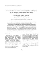
2.2. The workflow
The assessment of influence of interpolation
technique on the accuracy of DEM is carried
out according to the workflow presented in Fig.
1. The computation is done by using ArcGIS
software developed by ESRI [5].
The input data consists of two point sets: the
set of source (sample) points, and the set of
control (check) points. The control points are
evenly distributed and accurately measured. The
number of control points is about 0.5-1.0% of
the number of source points, but not less than 50.
Both point sets are imported into a
geodatabase as point feature classes having an
attribute field Elevation. The source point set is
then interpolated to create a raster DEM with a
relatively high resolution. The high resolution is

defined in order to eliminate the influence of
the output resolution on the accuracy of DEM.
The three described above interpolation
techniques are applied with varying parameters.


Source points Control points
Import to
geodatabase
Import to
geodatabase
Interpolation
Extract interpolated ele-
vations to control points
Compare interpolated
and control elevations
Compute RMSE
of DEM

Fig. 1. The workflow for assessing the influence of
interpolation technique on the accuracy of DEM by
using ArcGIS software.
In the next step, the elevations of
interpolated DEM are extracted to the control
points by using the ArcGIS's tool Extract
Values to Points. Thus, the output points will
have two attributes: the original Elevation, and
the extracted from DEM Int_Elevation. These
attributes are compared each with other to
derive the elevation difference

i
∆
for each point i:
ElevationElevationntI
i
−=∆ _
(2)
T.Q. Binh, N.T. Thuy / VNU Journal of Science, Earth Sciences 24 (2008) 176-183
179
The calculated differences are stored in a
newly created attribute field Elev_Diff.
In the final step, the RMSE (root mean
square error) of the interpolated DEM is
calculated by using the following formula:
∑
=
∆=
N
i
i
N
RMSE
1
2
1
, (3)
where N is the number of control points.
For automated execution of the workflow,
we have developed a model in the Model
Builder extension of ArcGIS software. For each

project, the user only has to change the
interpolation method and define its parameters
in order to re-run the entire process. The model
for IDW interpolation is presented in Fig. 2.

Fig. 2. Automated workflow execution
by using ArcGIS's Model Builder.
In the model in Fig. 2, the tools (denoted by
rectangles) are used as follows:
- IDW: interpolate source points into raster
DEM (it can be substituted by spline or kriging
for other interpolation techniques).
- Extract Values to Points: extract interpolated
elevations from the created DEM into the
control point feature class, and create a new
feature class (Extracted Pts).
- Add Field: add the Elev_Diff field to the
feature class Extracted Pts.
- Calculate Field: calculates the elevation
difference
i
∆
by using Eq. 2 and takes its
square value.
- Summary Statistics: calculates RMSE of
the interpolated DEM by using Eq. 3.
2.3. The study areas
This research is based on the survey data of
four topographic mapping projects: Thai
Nguyen, Go Cong Tay, Co Loa, and Duong

Lam. The projects are located in areas belonging
to different topography types. Table 1 lists the
short description of these projects. Since the
Thai Nguyen project is relatively large and
covers three types of topography, it was divided
into three subprojects: Plain Thai Nguyen, Hilly
Thai Nguyen, and Mountainous Thai Nguyen.
3. Results and discussion
The results of testing the influence of
interpolation technique on the accuracy of DEM
is presented in figures 3÷6 as combined graphs.
The horizontal axes represent interpolation
techniques with varying parameters, and the
vertical axes represent the root mean square
errors (RMSE) of DEMs in the unit of meter.
Fig. 3 uses the following notation:
- Plain, Hill, Mountain: the subprojects of
Thai Nguyen project that are located in plain,
hilly and mountainous areas respectively.
- S, C, E, G, L: spherical, circular, exponential,
gaussian, and linear models of experimental
variogram for the ordinary kriging interpolation
method.
- LD, QD: linear with linear drift and linear
with quadratic drift for the universal kriging
interpolation method.
T.Q. Binh, N.T. Thuy / VNU Journal of Science, Earth Sciences 24 (2008) 176-183
180
Table 1. Characteristics of the DEM projects
Project Location

Type of
topography
Survey method
Project's
area

Thai
Nguyen
South of Thai Nguyen Province.
21
o
18'÷22
o
00' N,
105
o
26'÷106
o
25' E
Combined plain,
hills, and
mountains
Digital photogrammetry by
using aerial photos at
1:30,000 scale. Source point
sampling interval ~25m
14,000 ha

Go Cong
Tay

South of Go Cong Tay Dist.,
Tien Giang Prov., Cuu Long
River Delta. 10
o
12'÷10
o
18' N,
106
o
32'÷106
o
40' E
Plain Digital photogrammetry by
using aerial photos at
1:22,000 scale. Source point
sampling interval ~30m
1,295 ha

Co Loa South-East of Dong Anh Dist.,
Hanoi. 21
o
06'÷21
o
08' N,
105
o
51'÷105
o
53' E
Plain Digital photogrammetry by

using aerial photos at 1:7,000
scale. Source point sampling
interval ~20m
245 ha

Duong Lam North-West of Son Tay Town,
Hanoi. 21
o
08'÷21
o
10' N,
105
o
27'÷105
o
29' E
Midland, hills,
mounds.
Total station in combination
with GPS. Source point
sampling interval 2÷30m
211 ha

RMSE
(m)
Thai Nguyen project
0
1
2
3

4
5
6
7
Plain
0.3306 0.3198 0.3108 0.2979 0.2912 0.2892 0.2905 0.6069 0.6026 0.5986 0.5952 0.59 0.5858 0.4144 0.4132 0.4125 0.4121 0.4114 0.4108 0.352 0.353 0.349 0.359 0.354 0.347 0.295
Hill
0.6265 0.6018 0.5807 0.5486 0.5276 0.5142 0.5055 0.6047 0.6147 0.6186 0.6208 0.623 0.624 0.5137 0.5136 0.5136 0.5136 0.5135 0.5135 0.691 0.691 0.485 0.686 0.691 0.683 0.536
Mountain
5.3331 4.9751 4.665 4.2384 4.065 4.0577 4.1235 2.408 2.4141 2.4184 2.4213 2.4252 2.4277 2.5358 2.5362 2.5366 2.537 2.5379 2.5388 5.882 5.908 5.806 6.088 5.940 5.623 2.966
1 1.5 2 3 4 5 6 0.05 0.1 0.15 0.2 0.3 0.4 0.05 0.1 0.15 0.2 0.3 0.4 S C E G L LD QD
Inverse Distance Weighted (with varying power
p)
Spline Regularized (with varying weight) Spline Tension (with varying weight) Kriging Ordinary Kriging
Univeral

Fig. 3. Results of testing DEM accuracy in the Thai Nguyen project.
RMSE
(m)

Co Loa project
0
0.1
0.2
0.3
0.4
0.5
RMSE
0.365 0.359 0.353 0.343 0.334 0.328 0.323 0.431 0.439 0.442 0.444 0.446 0.447 0.375 0.375 0.375 0.375 0.374 0.374 0.384 0.384 0.381 0.384 0.384 0.378 0.380
1 1.5 2 3 4 5 6 0.05 0.1 0.15 0.2 0.3 0.4 0.05 0.1 0.15 0.2 0.3 0.4 S C E G L LD QD

Inverse Distance Weighted (with varying
power p)
Spline Regularized (with varying
weight)
Spline Tension (with varying weight) Kriging Ordinary Kriging
Univeral

Fig. 4. Results of testing DEM accuracy in the Co Loa project.
T.Q. Binh, N.T. Thuy / VNU Journal of Science, Earth Sciences 24 (2008) 176-183
181
RMSE
(m)

Go Cong Tay project
0.00
0.02
0.04
0.06
0.08
0.10
RMSE
0.073 0.072 0.071 0.069 0.068 0.068 0.068 0.066 0.067 0.067 0.067 0.067 0.067 0.065 0.065 0.065 0.065 0.065 0.065 0.076 0.076 0.076 0.076 0.076 0.078 0.070
11.5234560.050.10.150.20.30.40.050.10.150.20.30.4SCEGLLDQD
Inverse Distance Weighted (with varying power p) Spline Regularized (with varying weight) Spline Tension (with varying weight) Kriging Ordinary Kriging
Univeral

Fig. 5. Results of testing DEM accuracy in the Go Cong Tay project.
RMSE
(m)
Duong Lam project

0.0
1.0
2.0
3.0
4.0
RMSE
0.409 0.383 0.367 0.356 0.360 0.366 0.371 3.347 3.559 3.687 3.759 3.820 3.820 1.143 1.093 1.067 1.051 1.028 1.010 0.279 0.278 0.278 0.378 0.284 0.346 0.346
1 1.5 2 3 4 5 6 0.05 0.1 0.15 0.2 0.3 0.4 0.05 0.1 0.15 0.2 0.3 0.4 S C E G L LD QD
Inverse Distance Weighted (with varying power
p)
Spline Regularized (with varying weight) Spline Tension (with varying weight) Kriging Ordinary Kriging
Univeral

Fig. 6. Results of testing DEM accuracy in the Duong Lam project.

3.1. The Thai Nguyen project
The results of testing DEM accuracy in the
Thai Nguyen project is presented in Fig. 3. For
this project, some remarks can be made as
follows:
- The error of DEM in the mountainous
subproject is much higher than those in the
plain and hilly subprojects. The reason is that
the elevation in mountainous areas strongly
varies, while the interpolation techniques can
account only for gradual changes over space.
- Among the three tested interpolation
techniques, the spline one (regularized or
tension) produces a much lower level of error in
the mountainous area.

- In the plain and hilly areas, all three
interpolation techniques give roughly comparable
results. The IDW is slightly better than others in
the plain area, while the kriging with
exponential model of semivariogram gives the
smallest RMSE (0.485m) in the hilly area.
- For the IDW interpolation, when the
power p increases, the error of DEM decreases,
but only by a small amount. Thus, for
improving the computational speed, one can
choose a relatively small value of p.
- For the spline interpolation, the tension
method has some advantages over the
regularized one in the plain and hilly areas.
Conversely, the regularized method is better in
the mountainous area.
- For the kriging interpolation, the ordinary
method using exponential model and the
universal method using linear model with
quadratic drift (QD) gives slightly smaller
RMSEs than other methods.
T.Q. Binh, N.T. Thuy / VNU Journal of Science, Earth Sciences 24 (2008) 176-183
182
3.2. The Co Loa project
The results of testing DEM accuracy in the
Co Loa project are presented in Fig. 4. It can be
readily seen that the graph for Co Loa is very
similar to the one for the plain area of Thai
Nguyen project. The IDW with a high value of
power p produces the best results, while the

spline regularized produces the worst.
However, due to the relatively flat characters of
topography in Co Loa, the interpolation
techniques do not have a strong effect on the
accuracy of DEM: the errors are within the
range from 0.32m to 0.38m except for the cases
of using the spline regularized method.
3.3. The Go Cong Tay project
Fig. 5 shows the DEM accuracy obtained in
the Go Cong Tay project. Since the project area
is very flat with elevation varied only from 0 to
4 m, the interpolation does not have much
influence, and the accuracy of DEM is very
high. All three interpolation techniques give
almost the same results, only the kriging one
shows a slightly higher level of error. Thus, for
a very flat area like the Go Cong Tay project,
the DEM accuracy isn't the main criterion for
choosing interpolation technique. The criterion
can be the computational speed (choosing IDW)
or the smoothness of the DEM (choosing spline).
3.4. The Duong Lam project
The results of testing DEM accuracy in the
Duong Lam project are shown in Fig. 6. Since
the survey method used in this project (total
station and GPS) differs from the one used in
other projects (digital photogrammetry), the
graph in Fig. 6 has a shape that is dissimilar to
those in figures 3÷5. The spline regularized
interpolation gives an extreme (abnormal)

RMSE of DEM, reaching 3.8 m, what is 13.7
times more than the error given by kriging
ordinary interpolation (0.278 m). The spline
tension interpolation is much better than the
spline regularized one, but still has an error
significantly large than other techniques. The
phenomenon can be explained as follows:
- In total station / GPS surveying, the
number of surveyed (sampled) points is very
limited. However, these points are very well
distributed, usually along breaklines where the
terrain surface sharply changes. The location of
each surveyed point is chosen manually by the
surveyors based on their interpretation of
topography and with some statistical meaning.
Meanwhile, the spline interpolation assumes
that the surface is smoothly passed through
sampled points, and thus it is not suitable for
the cases when most of these sample points are
allocated along breaklines.
- The abnormal error given by spline
regularized method is due to the fact that the
elevation peaks in the Duong Lam project were
already surveyed in the field by placing sample
points on them. The spline regularized tends to
interpolate the elevation beyond the surveyed
range, i.e. might give a elevation far higher than the
surveyed peaks that leads to the abnormal error.
- Since the distribution of sample points in
total station (or GPS) surveying has some

statistical meaning, kriging interpolation - the
most statistically rigid interpolation technique -
may have some advantages over others.
As it shows in Fig. 6, among the three
tested interpolation techniques, the kriging
ordinary with circular or exponential model has
the best accuracy (RMSE of 0.278 m). The IDW
interpolation is a bit less accurate with RMSE of
0.356 m. However, the IDW is much faster than
the kriging, and thus the choice of optimal
interpolation technique for the projects similar
to Duong Lam is not obvious, especially if they
cover a large area.
3.5 Recommendations on choosing interpolation
technique
From the above discussions, we have made
some recommendations on choosing appropriate
interpolation techniques based on the type of
topography and surveying method (Table 2).

T.Q. Binh, N.T. Thuy / VNU Journal of Science, Earth Sciences 24 (2008) 176-183
183
Table 2. Recommendations on choosing interpolation technique
Interpolation technique
Type of
topography
Survey method
Recommended Can be considered Not recommended

Mountainous Digital photogrammetry Spline regularized with

any weight
Spline tension Kriging

Hilly Digital photogrammetry IDW with power p > 3 Spline tension

Plain (Flat) Digital photogrammetry
IDW with power p=3÷5
Spline or kriging

Hilly or flat Total station / GPS Kriging ordinary with
exponential model for
small areas, IDW with
p=2÷3 for large areas
Spline, especially
spline regularized

If there are several topography types
available in the project area then the project can
be divided into subprojects with relatively
homogeneous type of topography. This can be
done automatically by analyzing the variation
of elevation by using statistical indicators, such
as variance or standard deviation.
4. Conclusions
Interpolation technique plays an important
role in achieving a high accuracy of DEM. The
influence of interpolation technique on the
DEM accuracy depends on the type of
topography, and the distribution of sample
points, what is directly related to the surveying

method. This research has examined three
interpolation techniques (IDW, spline, and
kriging) in four different survey projects. Based
on the analysis of obtained results, some
recommendations on choosing the optimal
interpolation technique has been made: for
mountainous areas, the spline regularized is the
most suitable; and for hilly and flat areas, the
IDW or kriging ordinary with exponential
model of variogram are recommended.
Acknowledgements
This paper was completed within the
framework of Fundamental Research Project
702406 funded by Vietnam Ministry of Science
and Technology.
References
[1] V. Chaplot et al., Accuracy of interpolation
techniques for the derivation of digital elevation
models in relation to landform types and data
density, Geomorphology 77 (2006) 126.
[2] I. M. El Hassan, Accuracy comparison of some
spline interpolation algorithms, Sudan Engineering
Society Journal 53 (2007) 59.
[3] R. Fencík, M. Vajsáblová, Parameters of
interpolation methods of creation of digital
model of landscape, The 9
th
AGILE Conference
on Geographic Information Science, Visegrad,
Hungary, 2006.

[4]
Z.L. Li, Q. Zhu, C. Gold, Digital terrain modeling:
principles and methodology, CRC Press, Boca
Raton, 2005.
[5] J. McCoy, K. Johnston, Using ArcGIS Spatial
Analyst, ESRI Press, Redland, CA, USA, 2001.
[6] L. Mitas, and H. Mitasova, General variational
approach to the interpolation problem, Computer
and Mathemathic Application 16 (1988) 983.
[7] M.A. Oliver, Kriging: a method of interpolation for
geographical information systems, International
Journal of Geographic Information Systems 4
(1990) 313.
[8] M. Peralvo, Influence of DEM interpolation
methods in drainage analysis, GIS Hydro 04,
Texas, USA, 2004.