Introduction to Practical Fluid Flow 2007 docx
Bạn đang xem bản rút gọn của tài liệu. Xem và tải ngay bản đầy đủ của tài liệu tại đây (3.89 MB, 208 trang )
//SYS21///INTEGRAS/B&H/IPF/FINAL_13-09-02/0750648856-CH000-PRELIMS.3D ± 1 ± [1±10/10] 23.9.2002
3:25PM
Introduction to Practical Fluid Flow
//SYS21///INTEGRAS/B&H/IPF/FINAL_13-09-02/0750648856-CH000-PRELIMS.3D ± 2 ± [1±10/10] 23.9.2002
3:25PM
This book is dedicated to my
wife Ellen
//SYS21///INTEGRAS/B&H/IPF/FINAL_13-09-02/0750648856-CH000-PRELIMS.3D ± 3 ± [1±10/10] 23.9.2002
3:25PM
Introduction to Practical
Fluid Flow
R.P. King
University of Utah
OXFORD AMSTERDAM BOSTON LONDON NEW YORK PARIS
SAN DIEGO SAN FRANCISCO SING APORE SYDNEY TOKYO
//SYS21///INTEGRAS/B&H/IPF/FINAL_13-09-02/0750648856-CH000-PRELIMS.3D ± 4 ± [1±10/10] 23.9.2002
3:25PM
Butterworth-Heinemann
An imprint of Elsevier Science
Linacre House, Jordan Hill, Oxford OX2 8DP
200 Wheeler Road, Burlington, MA 01803
First published 2002
Copyright
#
2002, R.P. King. All rights reserved
The right of R.P. King to be identified as the author of this work
has been asserted in accordance with the Copyright, Designs
and Patents Act 1988
No part of this publication may be
reproduced in any material form (including
photocopying or storing in any medium by electronic
means and whether or not transiently or incidentally
to some other use of this publication) without the
written permission of the copyright holder except
in accordance with the provisions of the Copyright,
Designs and Patents Act 1988 or under the terms of a
licence issued by the Copyright Licensing Agency Ltd,
90 Tottenham Court Road, London, England W1T 4LP.
Applications for the copyright holder's written permission
to reproduce any part of this publication should be
addressed to the publishers
British Library Cataloguing in Publication Data
King, R.P.
Introduction to practical fluid flow
1 Fluid dynamics
I Title
620.1
H
064
Library of Congress Cataloguing in Publication Data
King, R.P.
Introduction to practical fluid flow / R.P. King.
p. cm.
Includes bibliographical references and index.
ISBN 0 7506 4885 6
1 Fluid dynamics I Title
TA357 .K575 2002
620.1
H
064±dc21 2002029940
ISBN 0 7506 4885 6
For information on all Butterworth-Heinemann publications
visit our website at www.bh.com
Typeset by Integra Software Services Pvt. Ltd, Pondicherry 605 005, India
www.integra-india.com
Printed and bound in Italy
1 Introduction
1.1 Fluid flow in process engineering
1.2 Dimensions, units, and physical quantities
1.3 Properties of fluids
1.4 Fluid statics
1.5 Practice problems
1.6 Symbols
2 Flow of fluids in piping systems
2.1 Pressure drop in pipes and channels
2.2 The friction factor
2.3 Calculation of pressure gradient and
flowrate
2.4 The energy balance for piping systems
2.5 The effect of fittings in a pipeline
2.6 Pumps
2.7 Symbols
2.8 Practice problems
3 Interaction between fluids and particles
3.1 Basic concepts
3.2 Terminal settling velocity
3.3 Isolated isometric particles of arbitrary
shape
3.4 Symbols
3.5 Practice problems
4 Transportation of slurries
4.1 Flow of settling slurries in horizontal
pipelines
4.2 Four regimes of flow for settling slurries
4.3 Head loss correlations for separate flow
regimes
4.4 Head loss correlations based on a stratified
flow model
4.5 Flow of settling slurries in vertical pipelines
4.6 Practice problems
4.7 Symbols
5 Non-Newtonian slurries
5.1 Rheological properties of fluids
5.2 Newtonian and non-Newtonian fluids in
pipes with circular cross-section
5.3 Power-law fluids in turbulent flow in pipes
5.4 Shear-thinning fluids with Newtonian limit
5.5 Practice problems
5.6 Symbols used in this chapter
6 Sedimentation and thickening
6.1 Thickening
6.2 Concentration discontinuities in settling
slurries
6.3 Useful models for the sedimentation
velocity
6.4 Continuous cylindrical thickener
6.5 Simulation of the batch settling experiment
6.6 Thickening of compressible pulps
6.7 Continuous thickening of compressible
pulps
6.8 Batch thickening of compressible pulps
6.9 Practice problems
6.10 Symbols
Index
//SYS21///INTEGRAS/B&H/IPF/FINAL_13-09-02/0750648856-CH000-PRELIMS.3D ± 7 ± [1±10/10] 23.9.2002
3:25PM
Preface
This book deals with the transportation and handling of incompressible
fluids. This topic is important to most process engineers, because large quan-
tities of material are transported in the process engineering industries. The
emphasis of this book is on suspensions of particulate solids although the
basic principles of simple Newtonian fluid flow form the basis of the devel-
opment of models for the transportation of such material. Both settling
slurries and dense suspensions are considered. The latter invariably exhibit
non-Newtonian behavior. Transportation of slurries and other non-Newtonian
fluids is generally treated inadequately or perfunctorily in most of the texts
dealing with fluid transportation. This is a disservice to modern students in
chemical, metallurgical, civil, and mining engineering, where problems relat-
ing to the flow of slurries and other non-Newtonian fluids are commonly
encountered. Although the topics of non-Newtonian fluid flow and slurry
transportation are comprehensively covered in specialized texts, this book
attempts to consolidate these topics into a consistent treatment that follows
naturally from the conventional treatment of the transportation of incompres-
sible Newtonian fluids in pipelines. In order to keep the book to a reasonable
length, solid±liquid systems that are of interest in the mineral processing
industries are emphasized at the expense of the many other fluid types that
are encountered in the process industries in general. This reflects the particu-
lar interests of the author. However, the student should have no difficulty in
adapting the methods that are described here to other application areas. The
level is kept to that of undergraduate courses in the various process engineer-
ing disciplines, and this book could form the basis of a one-semester course
for students who have not necessarily had exposure to formal fluid
mechanics. This book could also usefully be adopted for students who have
or will take a course in fluid mechanics and who need to explore the typical
situations that they will meet as practising process engineers. The level of
mathematical analysis is consistent with that usually found in modern under-
graduate engineering curricula and is consistent with the need to describe the
subject matter at the level that is used in modern engineering analysis.
Modeling methods that are based on partial differential equations are used
in Chapter 6 because they are essential for the proper description of industrial
sedimentation and thickening processes where the solid concentration fre-
quently varies spatially and with time.
An important novel feature of this book is the unified treatment of the
friction factor information that is used to calculate the flow of all types of fluid
in round pipes. For each of the fluid types that are studied, the friction factor
is presented graphically in terms of the appropriate Reynolds number, the
dimensionless pipe diameter, the dimensionless flowrate and the dimension-
less flow velocity. Each of these graphical representations leads to the most
//SYS21///INTEGRAS/B&H/IPF/FINAL_13-09-02/0750648856-CH000-PRELIMS.3D ± 8 ± [1±10/10] 23.9.2002
3:25PM
convenient computational method for specific problems depending on what
information is specified and which variables must be computed. The same
problem-solving methods are used irrespective of the type of fluid be it
a simple Newtonian or a rheologically complex fluid such as those whose
behavior is described by the Sisko model. This uniformity should assist
students considerably in learning the basic principles and applying them
across a wide range of application areas.
The presentation of material is somewhat different to that found in most
textbooks in this field in that it is acknowledged that modern students of
engineering are computer literate. These students are accustomed to using
spreadsheets and other well-organized computational aids to tackle technical
problems. They do not rely only on calculators and almost never plot graphs
using pencil and paper. Few students submit handwritten reports. Conse-
quently, computer-oriented methods are emphasized throughout, and, where
appropriate, time-consuming or tedious computational processes are pre-
programmed and made available in the computational toolbox that accompanies
this text. This toolbox has been designed with care to ensure that it does not
provide point-and-click solutions to problems. Rather the student is encour-
aged to formulate a solution method for every specific problem, but the tools
in the toolbox make it feasible to tackle realistic problems that would be
simply too time consuming using manual computational methods or if the
student were required to generate the appropriate computer code. In any case,
students of process engineering are becoming less fluent in the traditional
computational languages Fortran, C, Basic, and Pascal that almost all could
use with some degree of proficiency during the last three decades of the
twentieth century. Now, engineering students are far more likely to be fluent
in computer languages such as Java and HTML and are more likely to be able
to create a website on the Internet than to be able to quickly and correctly
integrate a couple of differential equations numerically. Nevertheless, they
are well-attuned to using solution methods that are preprogrammed and
ready to be used. Students and instructors are encouraged to install the tool-
box and to explore its constituent tools before tackling any material in this
book. No specific programming skills are required of the student or the
instructor. The use of this modern problem-solving methodology makes it
possible to extend the treatment from a purely superficial level to a more
in-depth treatment and so equip the student to tackle, and successfully solve,
realistic engineering problems.
The quantitative models that are described in this text will surely change
and evolve over the years ahead as a result of continuing research and
investigational effort. However, the basic approach should be sufficiently
general to accommodate these developments. Because the computational
toolbox has an open-ended design, new models can be inserted with ease at
any time and it is intended that the toolbox should continue to expand well
into the future.
This book can be used as a reading text to support Internet-based
course delivery. This method has been used with success at the University
viii Preface
//SYS21///INTEGRAS/B&H/IPF/FINAL_13-09-02/0750648856-CH000-PRELIMS.3D ± 9 ± [1±10/10] 23.9.2002
3:25PM
of Utah, where such a course, supported by a fully equipped virtual labora-
tory, is now available. At the time of writing this course can be previewed at
.
Professor R.P. Chabbra and Professor Raj Rajamani made several useful
suggestions for improving the first draft of this book. These are gratefully
acknowledged.
R.P. King
Salt Lake City
Preface ix
//SYS21///INTEGRAS/B&H/IPF/FINAL_13-09-02/0750648856-CH000-PRELIMS.3D ± 10 ± [1±10/10] 23.9.2002
3:25PM
//SYS21///INTEGRAS/B&H/IPF/FINAL_13-09-02/0750648856-CH01.3D ± 1 ± [1±8/8] 23.9.2002 3:26PM
1
Introduction
1.1 Fluid flow in process engineering
Process engineering deals with the processing of large quantities of mater-
ial. In order to process materials, they must be transported to the process-
ing plant, and they must be transported from one unit operation to
another within the processing environment. Materials are usually trans-
ported in a fluid phase, because this is generally much easier and more
cost-effective than transportation as a solid. Liquids can be easily moved
through pipelines or open channels, and the energy that is required can be
conveniently delivered to the fluid using a pump. Gases too can be trans-
ported economically by pipeline, but this book deals exclusively with the
transportation of incompressible fluids. These include pure liquids, both
Newtonian and non-Newtonian, and suspensions of solid particles in
liquids that form slurries or pastes. Non-Newtonian fluids and suspensions
are commonly encountered by chemical, metallurgical, mining, and civil
engineers.
This book does not start from the usual definition of the fluid as a con-
tinuum from which the application of differential mass and momentum
balances leads to the equation of continuity and the Navier±Stokes equations.
The approach taken is macroscopic with an emphasis of solving problems of
practical engineering significance. The accompanying computational toolbox
provides the tools that are necessary to solve these problems with conveni-
ence, and the reader is expected to become familiar with the toolbox and its
contents.
1.2 Dimensions, units, and physical quantities
A variety of physical quantities of both the fluids and the equipment will
be used throughout this book. These quantities must be described quantita-
tively, for which sets of dimensions and units are required. For example,
the density of a fluid is an important quantity that will influence the
behavior of the fluid in most situations. The dimensions of density are
mass per unit volume M/L
3
. To give the density a numerical value, a set
of units must be selected for all the dimensions that are to be used. In this
book all units will be specified in the SI (Syste
Á
me International) system.
There is a good reason for this: the SI is the only practical set of units that
is coherent. This means that no conversion factors are ever required when
solving problems. This is in stark contrast to all other systems of units,
//SYS21///INTEGRAS/B&H/IPF/FINAL_13-09-02/0750648856-CH01.3D ± 2 ± [1±8/8] 23.9.2002 3:26PM
including the metric system, which require difficult-to-remember conver-
sion factors in almost every problem except perhaps only the most elemen-
tary and trivial. These older incoherent systems of units are now regarded
as being obsolete for the purposes of scientific and technical calculations.
The SI is based on a set of fundamental dimensions and units as shown in
Table 1.1. The precise size of each of the fundamental dimensions is defined
by reference to a unique physical entity. Because the size of the fundamental
dimensions that are used in the SI do not always conveniently match those
of the physical quantities that are encountered in practical problems, a set
of prefixes is defined which specify powers of 10 which multiply the
fundamental units as required for convenient specifications of the numerical
quantities. These are given in Table 1.3.
Clearly, the fundamental dimensions are not sufficient to describe all the
physical properties that are of interest, and a set of derived units that will be
of interest in this book is given in Table 1.2.
For example, the unit of density in the SI system is kg/m
3
.
The use of upper case letters in the unit abbreviations is restricted to those
units that are named for people. In Table 1.2 these are the newton (N), hertz
(Hz), pascal (Pa), joule (J), watt (W) and kelvin (K).
Some units that are outside the SI but which may be used with the SI are
given in Table 1.4. These outside units are not coherent with the SI and should
never be used in calculations. Convert any quantity in these units to the SI
unit before calculations begin.
The coherence of the SI system is demonstrated using the following simple
example. The energy that is required to transport a fluid from one location to
another can be calculated using the following equation, which is derived in
Chapter 2.
Energy required Change in potential energy Change in kinetic energy
specific volume of fluid  Change in pressure
Energy dissipated by friction:
Table 1.1 Fundamental dimensions in the SI and their units
Quantity Dimension SI unit Symboll
Length L meter m
Mass M kilogram kg
Time T second s
Electric current ampere A
Temperature K kelvin K
Quantity of a substance M gram-mole mol
Luminous intensity candela cd
Plane angle radian rad
Solid angle steradian sr
2 Introduction to Practical Fluid Flow
//SYS21///INTEGRAS/B&H/IPF/FINAL_13-09-02/0750648856-CH01.3D ± 3 ± [1±8/8] 23.9.2002 3:26PM
Such an energy balance is usually established for unit mass of fluid that flows.
The energy required will now be calculated using obsolete units and SI units
to demonstrate the advantages that are gained through the coherence of the
latter system.
Table 1.2 Some derived units in the SI
Quantity Dimension SI unit Name
Area L
2
m
2
Volume L
3
m
3
Velocity L=T m/s
Acceleration L=T
2
m/s
2
Angular velocity T
À1
rad/s
Force ML=T
2
N newton
Density M=L
3
kg/m
3
Frequency T
À1
Hz hertz
Pressure M=LT
2
Pa N=m
2
pascal
Specific energy L
2
=T
2
J/kg
Stress M=LT
2
N=m
2
Surface tension M=T
2
N/m
Work ML
2
=T
2
J Nm joule
Energy ML
2
=T
2
J Nm joule
Torque ML
2
=T
2
Nm
Power ML
2
=T
3
Nm=s J=s W watt
Entropy ML
2
=T
2
K J/K
Viscosity M=LT kg=ms Pa s
Mass flow M=T kg/s
Volume flow M
3
=T m
3
/s
Table 1.3 SI prefixes
Multiplying factor Prefix Symboll
10
12
tera T
10
9
giga G
10
6
mega M
10
3
kilo k
10
À2
centi c
10
À3
milli m
10
À6
micro m
10
À9
nano n
10
À12
pico p
Introduction 3
//SYS21///INTEGRAS/B&H/IPF/FINAL_13-09-02/0750648856-CH01.3D ± 4 ± [1±8/8] 23.9.2002 3:26PM
Table 1.5 Data for illustrative example
Data Obsolete units SI units
Initial elevation 3 ft above datum 0.9144 m
Final elevation 25 ft above datum 7.620 m
Initial velocity 2 ft/sec 0.6096 m/s
Final velocity 5 ft/sec 1.5240 m/s
Initial pressure 65 psig 4.482 Â 10
5
Pa
Final pressure 0 psig 0 Pa
Energy dissipated by friction 0.253 Btu/lb
m
5.88.48 J/kg
Density of fluid 62.4 lb
m
/ft
3
999.52 kg/m
3
Gravitational acceleration 32.2ft/sec
2
9.8081 m/s
2
Atmospheric pressure 740 mm mercury 98.664 kPa
The data for this example is set out in Table 1.5. The standard method for
setting out this calculation in the old system of units, as taught in many high
schools and universities in the United states, is as follows:
Energy required gz
final
À z
initial
1
2
V
2
final
À V
2
initial
P
final
À P
initial
F
32:2ft
s
2
25 À3ft
1lb
f
32:174 lb
m
ft=s
2
0:55
2
À 2
2
ft
2
=s
2
1lb
f
32:174 lb
m
ft=s
2
62:4lb
m
=ft
3
0 À65lb
f
=inch
2
12
2
inch
2
=ft
2
15:3 Btu=lb
m
1 ft-lb
f
1:284 Â10
À3
Btu
22:02 ft-lb
f
=lb
m
0:326 ft-lb
f
=lb
m
À 150:00 ft-lb
f
=lb
m
197:04 ft-lb
f
=lb
m
69:38 ft-lb
f
=lb
m
1:284 Â10
À3
Btu
1 ft-lb
f
0:0891 Btu=lb
m
Table 1.4 Some units outside the SI that are accepted for use with the SI
Name Symbol Value in SI units
minute (time) min 1 min 60 s
hour h 1 h 60 min 3600 s
day d 1 d 24 h 86400 s
degree (angle)
1
(p=180) rad
liter L 1 L 10
À3
m
3
metric ton t or tonne 1 t 1000 kg
bar bar 1 bar 0:1 Mpa 100 kPa 10
5
Pa
4 Introduction to Practical Fluid Flow
//SYS21///INTEGRAS/B&H/IPF/FINAL_13-09-02/0750648856-CH01.3D ± 5 ± [1±8/8] 23.9.2002 3:26PM
The above method is error prone, time consuming, and totally unnecessary if
the SI is used.
Using SI units, the calculation is set out in the following simple and
intuitive form by substituting the numerical values directly for the symbols
in the formulas.
Energy required 9:80817:620 À0:91440:51:524
2
À 0:096
2
0 À4:482 Â 10
5
999:52
588:48
206:8J=kg
Because SI units are used throughout, the units of the separate terms are
automatically consistent because of the coherence of the SI. Each term repre-
sents energy per unit mass so the answer is automatically in the SI unit for this
quantity, namely J/kg. No conversion factors are required.
This simple example suggests an effective strategy for dealing with calcula-
tions when the original data is specified in obsolete units. First convert all the
primary data into SI units. Perform all calculations in SI units which will never
require any conversion factors. The final answer is always in the appropriate
SI unit. If required, the final answer can be reported in any other system of
units by doing a single conversion out of SI to whatever unit is required. The
conversion of units into and out of the SI system is facilitated by the SI
conversion feature that is included in the FLUIDS toolbox on the CD-ROM
that is included with this book. This converter is illustrated in Figure 1.1.
1.3 Properties of fluids
Some elementary physical properties of fluids are discussed in this section.
1.3.1 Density and specific gravity
The density of a fluid is the mass of a unit volume of the fluid. For example,
water has a density of 998 kg/m
3
at 20
C. The density is usually represented
by the symbol .
Figure 1.1 SI unit converter in the FLUIDS toolbox
Introduction 5
//SYS21///INTEGRAS/B&H/IPF/FINAL_13-09-02/0750648856-CH01.3D ± 6 ± [1±8/8] 23.9.2002 3:26PM
The specific gravity of any substance is the ratio of the density of the substance
to the density of water. Specific gravity is usually represented by the symbol s.
s
water
1:1
1.3.2 Viscosity
Viscosity can be thought of as the internal stickiness of a fluid. When a fluid
flows, it deforms as one layer of fluid flows over another, and the rate of
deformation is governed by internal shearing stresses that are set up within
the fluid. The relationship between the shear stress and the rate of deform-
ation for many fluids is governed by the simple linear relationship
du
dy
1:2
Where represents shear stress, represents the viscosity, u is the velocity in
the fluid, and y is a spatial coordinate. The quantity du=dy is a velocity gradient
and can be interpreted as the rate at which strain or extension develops in the
fluid. Fluids that are described by equation 1.2 are known as Newtonian fluids.
Other types of behavior are possible, and fluids that deviate from equation 1.2
are called non-Newtonian. Such fluids are discussed in detail in Chapter 5.
The viscosity of a fluid is quite sensitive to the temperature, and liquids
show a strong decrease in viscosity as temperature increases.
1.3.3 Vapor pressure
All liquids show a greater or lesser tendency to vaporize and, if allowed to
come to equilibrium with its surroundings, a liquid will establish an equilib-
rium across the liquid±vapor interface. The pressure exerted by the molecules
of the fluid in the vapor phase is specific to each liquid, and the equilibrium
pressure is called the vapor pressure of the liquid. The vapor pressure is a
function of the temperature.
If the vapor pressure of a liquid exceeds the prevailing total pressure, the
liquid vaporizes rapidly by boiling. This phenomenon is commonly encoun-
tered with water, which has a vapor pressure of 101.3 kPa at 100
C. This is the
pressure that is exerted by the atmosphere of the earth at sea level. Water boils
briskly when in an open container at this temperature.
1.4 Fluid statics
When a fluid is stationary with respect to its container, there is no relative
motion between any neighboring elements in the fluid. However, conditions
in the fluid are not uniform, since it responds to the gravitational force field
and the pressure in the fluid increases in the direction of the force field (see
Figure 1.2). In the absence of any other forces, such as centrifugal force for
6 Introduction to Practical Fluid Flow
//SYS21///INTEGRAS/B&H/IPF/FINAL_13-09-02/0750648856-CH01.3D ± 7 ± [1±8/8] 23.9.2002 3:26PM
example, the pressure is uniform on any horizontal cross-section. The pres-
sure variation in the vertical direction is governed by a differential equation,
which can be derived simply by considering a force balance over a thin
imaginary horizontal slice in the body of the fluid.
Since the fluid is in equilibrium, the weight of the slice of liquid must be
balanced by the net pressure force,
P
zÁz
A ÁzA
f
g P
z
A 1:3
P
zÁz
À P
z
Áz
À
f
g 1:4
where
f
is the density of the fluid.
In the limit as Áz 3 0, this generates the differential equation
dP
dz
À
f
g 1:5
Over modest depths in the gravitational fields of the earth,
f
and g are
constant, and this equation can be integrated to give
P À
f
gz constant 1:6
If h is the distance below the free surface of the fluid, the pressure is given by
P g
f
h atmospheric pressure 1:7
The unit of pressure in the SI is the pascal (Pa), which is identical to N/m
2
.
1.5 Practice problems
1. Water of density 62:4 lbs=ft
3
flows at velocity V 4:2ft=s through a
pipe of diameter D 6 inches. The viscosity of the water is 1 centipoise.
Calculate the value of the Reynolds number
Re
DV
2. Show that the Reynolds number has no dimensions.
Force =
P
z+∆z
A
Force =
P
z
A
∆z
Figure 1.2 Vertical variation of pressure in a static fluid
Introduction 7
//SYS21///INTEGRAS/B&H/IPF/FINAL_13-09-02/0750648856-CH01.3D ± 8 ± [1±8/8] 23.9.2002 3:26PM
3. Calculate the pressure 10 ft below the surface of a swimming pool situated
at sea level. Atmospheric pressure is 1005 millibar and the density of
water is 998 kg/m
3
.
1.6 Symbols used in this chapter
F Energy dissipation by friction J/kg
g Gravitational field
K Kelvin
L Length
M Mass
P Pressure
s Specific gravity
T Time
u Velocity in fluid
V Velocity
z Vertical height
Viscosity
Density
Shear stress
Bibliography
The United States standard for SI units is defined by the National Institute for
Standards and Technology (NIST). At the time of writing a summary of this
standard is available at />Factors for converting obsolete units to SI units are given by Lees (1968).
Reference
Lees, F.P. (1968). An SI unit conversion table for chemical engineers. The Chemical
Engineer, October 1968, pp. CE341±CE344.
8 Introduction to Practical Fluid Flow
//SYS21///INTEGRAS/B&H/IPF/FINAL_13-09-02/0750648856-CH02.3D ± 9 ± [9±54/46] 23.9.2002 4:35PM
2
Flow of fluids in piping systems
2.1 Pressure drop in pipes and channels
When a fluid flows through a pipe, it transfers momentum to the pipe wall. In
other words the pipe wall experiences a force in the direction in which the
fluid is moving. This force is best thought of as a frictional drag on the inside
of the pipe wall. This concept is illustrated in Figure 2.1. The frictional drag
acts along the inner surface of the pipe wall and appears as a shearing stress.
The fluid against the inner pipe surface experiences this shearing stress which
resists the motion of the fluid. The force on the inside wall of the pipe is
related to the shearing stress through the relationship
Force DL
w
N 2:1
where D is the pipe diameter and L is the length of the pipe. The shearing
stress on the wall,
w
, is determined primarily by the velocity of the fluid in
the pipe but it is also a function of the properties of the fluid (density and
viscosity). Obviously it is reasonable to expect that a more viscous fluid will
exert a greater shearing stress than a mobile fluid such as water. The shear
stress is related to the fluid velocity through an empirical equation
w
1
2
f
"
V
2
f N=m
2
2:2
where
"
V is the average velocity of the fluid in the pipe,
f
is the fluid density
and f is a variable called the friction factor. The friction factor is a function of
the properties of the fluid but its value depends mostly on the state of
turbulence in the fluid. Interestingly, the friction factor decreases as the fluid
becomes more intensely turbulent dropping from a value around 0.012 for
D
L
Velocity profile develops in the fluid.
Fluid velocity is zero at the pipe wall.
Shear stress is proportional to the velocity gradient
at the wall surface
Fluid moving inside pipe drags against
the inside of the pipe wall
Figure 2.1 Origin of the force that is exerted by the flowing fluid on the pipe
//SYS21///INTEGRAS/B&H/IPF/FINAL_13-09-02/0750648856-CH02.3D ± 10 ± [9±54/46] 23.9.2002 4:35PM
fluids that flow in a slow orderly manner that is barely turbulent inside
a smooth pipe to values that are only about one tenth of that value when
the fluid moves very fast inside the pipe and is intensely turbulent.
The average velocity of the fluid is related to the total volumetric flowrate Q by
"
V
Q
4
D
2
m=s 2:3
Substitution of equation 2.2 into equation 2.1 gives
Force DL
1
2
f
"
V
2
f N 2:4
The force is generated by the pressure gradient along the pipe. When the fluid
is flowing steadily equation 2.4 can be converted into a form that gives the
pressure gradient due to friction (PGDTF) as the fluid flows through the pipe
under steady conditions.
PGDTF À
ÁP
f
L
Force
4
D
2
L
2
D
f
"
V
2
f
4
w
D
N=m
2
2:5
The symbol ÁP
f
in equation 2.5 represents the pressure drop that the flowing
fluid experiences due only to the fractional drag on the pipe wall. The
pressure decreases in the direction of flow so that ÁP
f
has a negative numer-
ical value. This makes PGDTF a positive quantity. Equation 2.5 provides
a method for the experimental determination of the friction factor, f, because
PGDTF can be measured in the laboratory.
The energy dissipated by the frictional drag can be calculated from the
force exerted by the fluid on the pipe wall. The energy dissipation is calcu-
lated as energy used per unit mass of fluid.
F
Force ÂL
4
D
2
L
f
J=kg 2:6
Using equations 2.4 and 2.5 this becomes
F 2f
"
V
2
L
D
ÀÁP
f
f
J=kg 2:7
It is common practice to express pressure in terms of the equivalent height of a
column of fluid in the gravitational field of the earth.
ÀÁP
f
g
f
h
f
2:8
h
f
is called the head loss due to friction
h
f
2
f
"
V
2
g
L
D
2:9
10 Introduction to Practical Fluid Flow
//SYS21///INTEGRAS/B&H/IPF/FINAL_13-09-02/0750648856-CH02.3D ± 11 ± [9±54/46] 23.9.2002 4:35PM
The head loss due to friction is sometimes also expressed in terms of the
number of velocity heads, N
vh
, that are lost. A velocity head is defined to be
the quantity
"
V
2
/2g so that
h
f
N
vh
"
V
2
2g
2:10
Comparing this with equation 2.9
N
vh
4f
L
D
2:11
Whenever the pipe has a cross-section that is not circular but the pipe still
runs full, the diameter D in all of the above formulas should be replaced by
the hydraulic mean diameter which is defined by
D
H
4 Âflow cross-sectional area
wetted perimeter
2:12
2.2 The friction factor
Experiments have shown that the friction factor can be correlated uniquely
with the Reynolds number calculated for the fluid as it flows inside the
channel.
Re
D
"
V
f
f
2:13
A large amount of data obtained experimentally using many different
fluids in pipes having diameters differing by orders of magnitude have been
assembled into the so-called friction-factor chart. This chart is shown in Figure
2.2 and it is probably the most widely used chart by engineers who deal with
fluid flow problems. It is important to understand that the friction factor plot
represents experimentally determined data and does not have a priori theor-
etical foundation. It appears in virtually every text book that covers hydro-
dynamics and fluid flow. It has been published in several sizes and prior to
the personal computer era it was common to read values directly from the
graph with the attendant lack of precision. Now computer versions of
the friction factor chart are readily available and the chart is included in the
FLUIDS toolbox that is included on the CD-ROM that accompanies this book.
Empirical expressions have been established that summarize these graphs
and the most widely used equation is
1
f
p
1:74 lnRe
f
p
À0:40 2:14
Equation 2.14 applies only when the inside of the pipe wall is smooth and the
fluid is turbulent in the pipe which occurs when Re > 2000.
Flow of fluids in piping systems 11
//SYS21///INTEGRAS/B&H/IPF/FINAL_13-09-02/0750648856-CH02.3D ± 12 ± [9±54/46] 23.9.2002 4:35PM
When the inside of the pipe wall is rough the friction factor increases and
equation 2.14 is modified to
1
f
p
À1:74 ln 0:338
e
D
1
Re
f
p
23
À0:4
1
f
p
À1:74 ln 0:27
e
D
1:25
Re
f
p
23
2:15
e/D is a measure of the surface roughness relative to the pipe diameter. e is the
average height of any rough features on the inner surface. Typical values of
the surface roughness for some common materials are given in Table 2.1.
Equation 2.15 is commonly referred to as the Colebrook equation.
Equations 2.14 and 2.15 are not particularly convenient to use because
neither gives the value of f as an explicit function of the Reynolds number, Re.
An approximate formula for the friction factor over a restricted range of
Reynolds number that is often used because it does give f as an explicit
function of Re, is the Blasius equation
f 0:079 Re
À0:25
2:16
This equation is a reasonably good representation of the data for smooth pipes
over the range 2000 < Re < 100 000.
When Re < 2000 the flow is laminar and the friction factor is given by
f
16
Re
2:17
This relationship is derived in Section 5.2.1
10
–2
Reynolds number
Re
Friction factor
f
Friction factor for Newtonian fluids
10
–3
10
3
10
4
10
5
10
6
10
7
e/D = 0.0500
e/D = 0.0250
e/D = 0.0100
e/D = 0.0050
e/D = 0.0025
e/D = 0.0010
e/D = 0.0005
e/D = 0.0000
e/D = 0.0002
e/D = 0.0001
Figure 2.2 Friction factor plotted against the pipe Reynolds number. These graphs
were generated using equation 2.15
12 Introduction to Practical Fluid Flow
//SYS21///INTEGRAS/B&H/IPF/FINAL_13-09-02/0750648856-CH02.3D ± 13 ± [9±54/46] 23.9.2002 4:35PM
2.3 Calculation of pressure gradient and flowrate
It should be clear that the correlations for the friction factor f given in the
friction-factor chart make it possible to calculate the pressure gradient in a
pipe whenever the flowrate and the pipe diameter are known. It is simply
a matter of calculating the Reynolds number Re and reading the correspond-
ing friction factor on the chart. The corresponding pressure gradient due to
friction can be calculated using Equation 2.5. Reading values from the friction-
factor chart is not particularly accurate but accurate values can be easily and
conveniently obtained from the FLUIDS software package on the CD-ROM
that accompanies this book.
Illustrative example 2.1
Calculate the pressure gradient due to friction when water flows through a
smooth 10 cm diameter pipe at 1.5 m/s. Assume this data for the water:
w
1000 kg/m
3
and
f
0:001 kg/ms.
Re
D
"
V
f
f
0:10 Â1:5 Â 1000
0:001
1:5 Â 10
5
The friction factor plot can be read from the friction-factor chart or pre-
ferably obtained from the FLUIDS toolbox using the single-phase fluid friction
Table 2.1 Effective roughness of various surfaces (Source: Darby, 1996)
Material Condition Roughness range
(mm)
Recommended
value (mm)
Drawn copper, brass or
stainless steel
New 0.0015±0.01 0.002
Commercial steel New 0.02±0.1 0.045
Light rust 0.15±1.0 0.3
General rust 1±3 2.0
Iron Wrought, new 0.045 0.045
Cast, new 0.25±1 0.3
Galvanized 0.025±0.15 0.15
Asphalt-coated 0.1±1.0 0.15
Sheet metal Ducts, smooth joints 0.02±0.1 0.03
Concrete Very smooth 0.025±0.18 0.04
Wood floated, brushed 0.2±0.8 0.3
Rough, visible form marks 0.8±2.5 2.0
Wood Stave 0.25±1.0 0.5
Glass and plastic Drawn tubing 0.0015±0.01 0.002
Rubber Smooth tubing 0.006±0.07 0.01
Wire-reinforced 0.3±4.0 1.0
Flow of fluids in piping systems 13
//SYS21///INTEGRAS/B&H/IPF/FINAL_13-09-02/0750648856-CH02.3D ± 14 ± [9±54/46] 23.9.2002 4:35PM
factor screen as shown in Figure 2.3. The value for f at the specified value of
Re is 0.0040.
The pressure gradient due to friction is obtained from equation 2.5
PGDTF
ÀÁP
f
L
2
f
"
V
2
f
D
2 Â1000 Â 1:5
2
 0:00401
0:1
180:4Pa=m
Illustrative example 2.2
Calculate the increase in the pressure gradient due to friction if the inside of
the pipe wall has roughness 0:1 mm.
This can be done conveniently by changing the `Pipe wall roughness' entry
on the data form as shown in Figure 2.4 and calculating the new value of the
friction factor which is f 0:00518 as shown.
The new value of PGDTF is
PGDTF
2 Â1000 Â 1:5
2
 0:00518
0:1
233:1Pa=m
Note the significant increase in pressure gradient due to this comparatively
small increment in roughness of the wall surface.
The conventional friction-factor chart is not at all convenient for the calcu-
lation of the flowrate when the available pressure gradient and the pipe
diameter are known and an alternative method is developed here that facili-
tates calculations of this type.
Figure 2.3 Data input screen to calculate friction factor using the FLUIDS toolbox
14 Introduction to Practical Fluid Flow
//SYS21///INTEGRAS/B&H/IPF/FINAL_13-09-02/0750648856-CH02.3D ± 15 ± [9±54/46] 23.9.2002 4:35PM
The relationship between f and Re shown in Figure 2.2 is plotted as a series
of graphs of f against (Re
2
f )
1/3
as shown in Figure 2.5. An explicit method for
the calculation of the flowrate through a pipe when the diameter and avail-
able pressure gradient are known can be readily developed using this plot.
When the fluid is flowing steadily the friction factor is related to the pressure
gradient by equation 2.5 which gives
"
V
2
f
PGDTF ÂD
2
f
2:18
Figure 2.4 Specification of parameters for illustrative example 2.2
Dimensionless diameter D*=( )
Re f
2 1/3
Friction factor
f
10
–3
e/D = 0.0500
e/D = 0.0250
e/D = 0.0100
e/D = 0.0050
e/D = 0.0025
e/D = 0.0010
e/D = 0.0005
e/D = 0.0000
e/D = 0.0002
e/D = 0.0001
10
1
10
2
10
3
10
4
10
–2
Figure 2.5 Friction factor plotted against the dimensionless pipe diameter. Use this
chart if the pipe diameter and the PGDTF are known
Flow of fluids in piping systems 15