Limits on Interest Rate Rules in the ISModel potx

Limits on
InterestRate Rules
in the IS Model
William Kerr and Robert G. King
M
any central banks have long used a short-term nominal interest rate
as the main instrument through which monetary policy actions are
implemented. Some monetary authorities have even viewed their
main job as managing nominal interest rates, by using an interest rate rule for
monetary policy. It is therefore important to understand the consequences of
such monetary policies for the behavior of aggregate economic activity.
Over the past several decades, accordingly, there has been a substantial
amount of research on interest rate rules.
1
This literature finds that the fea-
sibility and desirability of interest rate rules depends on the structure of the
model used to approximate macroeconomic reality. In the standard textbook
Keynesian macroeconomic model, there are few limits: almost any interest rate
Kerr is a recent graduate of the University of Virginia, with bachelor’s degrees in system
engineering and economics. King is A. W. Robertson Professor of Economics at the Uni-
versity of Virginia, consultant to the research department of the Federal Reserve Bank of
Richmond, and a research associate of the National Bureau of Economic Research. The
authors have received substantial help on this article from Justin Fang of the University of
Pennsylvania. The specific expectational IS schedule used in this article was suggested by
Bennett McCallum (1995). We thank Ben Bernanke, Michael Dotsey, Marvin Goodfriend,
Thomas Humphrey, Jeffrey Lacker, Eric Leeper, Bennett McCallum, Michael Woodford, and
seminar participants at the Federal Reserve Banks of Philadelphia and Richmond for helpful
comments. The views expressed are those of the authors and do not necessarily reflect those
of the Federal Reserve Bank of Richmond or the Federal Reserve System.
1
This literature is voluminous, but may be usefully divided into four main groups. First,

there is work with small analytical models with an “IS-LM” structure, including Sargent and Wal-
lace (1975), McCallum (1981), Goodfriend (1987), and Boyd and Dotsey (1994). Second, there
are simulation studies of econometric models, including the Henderson and McKibbin (1993) and
Taylor (1993) work with larger models and the Fuhrer and Moore (1995) work with a smaller one.
Third, there are theoretical analyses of dynamic optimizing models, including work by Leeper
(1991), Sims (1994), and Woodford (1994). Finally, there are also some simulation studies of
dynamic optimizing models, including work by Kim (1996).
Federal Reserve Bank of Richmond Economic Quarterly Volume 82/2 Spring 1996
47
48 Federal Reserve Bank of Richmond Economic Quarterly
policy can be used, including some that make the interest rate exogenously
determined by the monetary authority. In fully articulated macroeconomic
models in which agents have dynamic choice problems and rational expecta-
tions, there are much more stringent limits on interest rate rules. Most basically,
if it is assumed that the monetary policy authority attempts to set the nominal
interest rate without reference to the state of the economy, then it may be
impossible for a researcher to determine a unique macroeconomic equilibrium
within his model.
Why are such sharply different answers about the limits to interest rate rules
given by these two model-building approaches? It is hard to reach an answer to
this question in part because the modeling strategies are themselves so sharply
different. The standard textbook model contains a small number of behavioral
relations—an IS schedule, an LM schedule, a Phillips curve or aggregate supply
schedule, etc.—that are directly specified. The standard fully articulated model
contains a much larger number of relations—efficiency conditions of firms and
households, resource constraints, etc.—that implicitly restrict the economy’s
equilibrium. Thus, for example, in a fully articulated model, the IS schedule
is not directly specified. Rather, it is an outcome of the consumption-savings
decisions of households, the investment decisions of firms, and the aggregate
constraint on sources and uses of output.

Accordingly, in this article, we employ a series of macroeconomic models
to shed light on how aspects of model structure influence the limits on interest
rate rules. In particular, we show that a simple respecification of the IS sched-
ule, which we call the expectational IS schedule, makes the textbook model
generate the same limits on interest rate rules as the fully articulated models.
We then use this simple model to study the design of interest rate rules with
nominal anchors.
2
If the monetary authority adjusts the interest rate in response
to deviations of the price level from a target path, then there is a unique equi-
librium under a wide range of parameter choices: all that is required is that the
authority raise the nominal rate when the price level is above the target path
and lower it when the price level is below the target path. By contrast, if the
monetary authority responds to deviations of the inflation rate from a target
path, then a much more aggressive pattern is needed: the monetary authority
must make the nominal rate rise by more than one-for-one with the inflation
rate.
3
Our results on interest rate rules with nominal anchors are preserved
when we further extend the model to include the influence of expectations on
aggregate supply.
2
An important recent strain of literature concerns the interaction of monetary policy and
fiscal policy when the central bank is following an interest rate rule, including work by Leeper
(1991), Sims (1994) and Woodford (1994). The current article abstracts from consideration of
fiscal policy.
3
Our results are broadly in accord with those of Leeper (1991) in a fully articulated model.
W. Kerr and R. G. King: Limits on Interest Rate Rules 49
1. INTEREST RATE RULES IN THE TEXTBOOK MODEL

In the textbook IS-LM model with a fixed price level, it is easy to implement
monetary policy by use of an interest rate instrument and, indeed, with a pure
interest rate rule which specifies the actions of the monetary authority entirely
in terms of the interest rate. Under such a rule, the monetary sector simply
serves to determine the quantity of nominal money, given the interest rate
determined by the monetary authority and the level of output determined by
macroeconomic equilibrium. Accordingly, as in the title of this article, one may
describe the analysis as being conducted within the “IS model” rather than in
the “IS-LM model.”
In this section, we first study the fixed-price IS model’s operation under a
simple interest rate rule and rederive the familiar result discussed above. We
then extend the IS model to consider sustained inflation by adding a Phillips
curve and a Fisher equation. Our main finding carries over to the extended
model: in versions of the textbook model, pure interest rate rules are admissible
descriptions of monetary policy.
Specification of a Pure Interest Rate Rule
We assume that the “pure interest rate rule” for monetary policy takes the form
R
t
= R + x
t
, (1)
where the nominal interest rate R
t
contains a constant average level R.
(Throughout the article, we use a subscript t to denote the level of the variable
at date t of our discrete time analysis and an underbar to denote the level of the
variable in the initial stationary position). There are also exogenous stochastic
components to interest rate policy, x
t

, that evolve according to
x
t
= ρx
t−1
+ ε
t
, (2)
with ε
t
being a series of independently and identically distributed random vari-
ables and ρ being a parameter that governs the persistence of the stochastic
components of monetary policy. Such pure interest rate rules contrast with
alternative interest rate rules in which the level of the nominal interest rate
depends on the current state of the economy, as considered, for example, by
Poole (1970) and McCallum (1981).
The Standard IS Curve and the Determination of Output
In many discussions concerning the influence of monetary disturbances on real
activity, particularly over short periods, it is conventional to view output as
determined by aggregate demand and the price level as predetermined. In such
discussions, aggregate demand is governed by specifications closely related to
the standard IS function used in this article,
y
t
− y = −s

r
t
−r


, (3)
50 Federal Reserve Bank of Richmond Economic Quarterly
where y denotes the log-level of output and r denotes the real rate of interest.
The parameter s governs the slope of the IS schedule as conventionally drawn
in (y, r ) space: the slope is s
−1
so that a larger value of s corresponds to a
flatter IS curve. It is conventional to view the IS curve as fairly steep (small s),
so that large changes in real interest rates are necessary to produce relatively
small changes in real output.
With fixed prices, as in the famous model of Hicks (1937), nominal and
real interest rates are the same (R
t
= r
t
). Thus, one can use the interest rate
rule and the IS curve to determine real activity. Algebraically, the result is
y
t
− y = −s

(R −r) + x
t

. (4)
A higher rate of interest leads to a decline in the level of output with an “interest
rate multiplier” of s.
4
Poole (1970) studies the optimal choice of the monetary policy instrument
in an IS-LM framework with a fixed price level; he finds that it is optimal

for the monetary authority to use an interest rate instrument if there are pre-
dominant shocks to money demand. Given that many central bankers perceive
great instability in money demand, Poole’s analytical result is frequently used
to buttress arguments for casting monetary policy in terms of pure interest rate
rules. From this standpoint it is notable that in the model of this section—which
we view as an abstraction of a way in which monetary policy is frequently
discussed—the monetary sector is an afterthought to monetary policy analysis.
The familiar “LM” schedule, which we have not as yet specified, serves only
to determine the quantity of money given the price level, real income, and the
nominal interest rate.
Inflation and Inflationary Expectations
During the 1950s and 1960s, the simple IS model proved inappropriate for
thinking about sustained inflation, so the modern textbook presentation now
includes additional features. First, a Phillips curve (or aggregate supply sched-
ule) is introduced that makes inflation depend on the gap between actual and
capacity output. We write this specification as
π
t
= ψ (y
t
− y), (5)
where the inflation rate π is defined as the change in log price level, π
t
≡
P
t
− P
t−1
. The parameter ψ governs the amount of inflation (π) that arises
from a given level of excess demand. Second, the Fisher equation is used to

describe the relationship between the real interest rate (r
t
) and the nominal
interest rate (R
t
),
R
t
= r
t
+ E
t
π
t+1
, (6)
4
Many macroeconomists would prefer a long-term interest rate in the IS curve, rather than
a short-term one, but we are concentrating on developing the textbook model in which this
distinction is seldom made explicit.
W. Kerr and R. G. King: Limits on Interest Rate Rules 51
where the expected rate of inflation is E
t
π
t+1
. Throughout the article, we
use the notation E
t
z
t+s
to denote the date t expectation of any variable z at

date t + s.
To study the effects of these two modifications for the determination of
output, we must solve for a reduced form (general equilibrium) equation that
describes the links between output, expected future output, and the nominal
interest rate. Closely related to the standard IS schedule, this specification is
y
t
− y = −s[(R −r) + x
t
] + sψ [E
t
y
t+1
− y]. (7)
This general equilibrium locus implies that there is a difference between tempo-
rary and permanent variations in interest rates. Holding E
t
y
t+1
constant at y, as
is appropriate for temporary variations, we have the standard IS curve determi-
nation of output as above. With E
t
y
t+1
= y
t
, which is appropriate for permanent
disturbances, an alternative general equilibrium schedule arises which is “flat-
ter” in (y, R) space than the conventional specification. This “flattening” reflects

the following chain of effects. When variations in output are expected to occur
in the future, they will be accompanied by inflation because of the positive
Phillips curve link between inflation and output. With the consequent higher
expected inflation at date t, the real interest rate will be lower and aggregate
demand will be higher at a particular nominal interest rate.
Thus, “policy multipliers” depend on what one assumes about the adjust-
ment of inflation expectations. If expectations do not adjust, the effects of
increasing the nominal interest rate are given by
∆y
∆R
= −s and
∆π
∆R
= −sψ ,
whereas the effects if expectations do adjust are
∆y
∆R
= −s/[1 − sψ ] and
∆π
∆R
= −sψ /[1 − sψ ]. At the short-run horizons that the IS model is usually
thought of as describing best, the conventional view is that there is a steep
IS curve (small s) and a flat Phillips curve (small ψ ) so that the denominator
of the preceding expressions is positive. Notably, then, the output and inflation
effects of a change in the interest rate are of larger magnitude if there is an
adjustment of expectations than if there is not. For example, a rise in the
nominal interest rate reduces output and inflation directly. If the interest rate
change is permanent (or at least highly persistent), the resulting deflation will
come to be expected, which in turn further raises the real interest rate and
reduces the level of output.

There are two additional points that are worth making about this extended
model. First, when the Phillips curve and Fisher equations are added to the
basic Keynesian setup, one continues to have a model in which the monetary
sector is an afterthought. Under an interest rate policy, one can use the LM
equation to determine the effects of policy changes on the stock of money,
but one need not employ it for any other purpose. Second, higher nominal
interest rates lead to higher real interest rates, even in the long run. In fact,
because there is expected deflation which arises from a permanent increase in
52 Federal Reserve Bank of Richmond Economic Quarterly
the nominal interest rate, the real interest rate rises by more than one-for-one
with the nominal rate.
5
Rational Expectations in the Textbook Model
There has been much controversy surrounding the introduction of rational ex-
pectations into macroeconomic models. However, in this section, we find that
there are relatively minor qualitative implications within the model that has
been developed so far. In particular, a monetary authority can conduct an unre-
stricted pure interest rate policy so long as we have the conventional parameter
values implying sψ < 1. In the rational expectations solution, output and infla-
tion depend on the entire expected future path of the policy-determined nominal
interest rate, but there is a “discounting” of sorts which makes far-future values
less important than near-future ones.
To determine the rational expectations solution for the standard Keynesian
model that incorporates an IS curve (3), a Phillips curve (5), and the Fisher
equation (6), we solve these three equations to produce an expectational dif-
ference equation in the inflation rate,
π
t
= −sψ [(R
t

− r) −E
t
π
t+1
], (8)
which links the current inflation rate π
t
to the current nominal interest rate and
the expected future inflation rate.
6
Substituting out for π
t+1
using an updated
version of this expression, we are led to a forward-looking description of cur-
rent inflation as related to the expected future path of interest rates and a future
value of the inflation rate,
π
t
= −sψ (R
t
− r) −(sψ )
2
E
t
(R
t+1
− r) . . .
−(sψ )
n
E

t
(R
t+n−1
−r) + (sψ )
n
E
t
π
t+n
. (9)
For short-run analysis, the conventional assumption is that there is a steep IS
curve (small s) because goods demand is not too sensitive to interest rates and a
flat Phillips curve (small ψ ) because prices are not too responsive to aggregate
demand. Taken together, these conditions imply that sψ < 1 and that there is
substantial “discounting” of future interest rate variations and of the “terminal
inflation rate” E
t
π
t+n
: the values of the exogenous variable R and endogenous
variable π that are far away matter much less than those nearby. In particular, as
we look further and further out into the future, the value of long-term inflation,
E
t
π
t+n
, exerts a less and less important influence on current inflation.
5
This implication is not a particularly desirable one empirically, and it is one of the factors
that leads us to develop the models in subsequent sections.

6
Alternatively, we could have worked with the difference equation in output (7), since the
Phillips curve links output and inflation, but (8) will be more useful to us later when we modify
our models to include price level and inflation targets.
W. Kerr and R. G. King: Limits on Interest Rate Rules 53
Using this conventional set of parameter values and making the standard
rational expectations solution assumption that the inflation process does not
contain explosive “bubble components,” the monetary authority can employ
any pure nominal interest rate rule.
7
Using the assumed form of the pure in-
terest rate policy rule, (1) and (2), the inflation rate is
π
t
= −sψ

1
1 − sψ
(R
− r) +
1
1 −sψρ
x
t

. (10)
Thus, a solution exists for a wide range of persistence parameters in the policy
rule (all ρ < (sψ )
−1
). Notably, it exists for ρ = 1, in which variations in the

random component of interest rates are permanent and the “policy multipliers”
are equal to those discussed in the previous subsection.
8
2. EXPECTATIONS AND THE IS SCHEDULE
Developments in macroeconomics over the last two decades suggest the impor-
tance of modifying the IS schedule to include a dependence of current output
on expected future output. In this section, we introduce such an “expectational
IS schedule” into the model and find that there are important limits on interest
rate rules. We conclude that one cannot or should not use a pure interest rate
rule, i.e., one without a response to the state of the economy.
Modifying the IS Schedule
Recent work on consumption and investment choices by purposeful firms and
households suggests that forecasts of the future enter importantly into these
decisions. These theories suggest that the conventional IS schedule (3) should
be replaced by an alternative, expectational IS schedule (EIS schedule) of the
form
y
t
− E
t
y
t+1
= −s

r
t
−r

. (11)
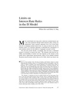
Figure 1 draws this schedule in (y, r) space, i.e., we graph

r
t
= r −
1
s
(y
t
− E
t
y
t+1
).
7
More precisely, we require that the policy rule must result in a finite inflation rate, i.e.,
|π
t
| = |sψ


∞
j=0
(sψ )
j
E
t
(R
t+j
−r)

| < ∞. Since sψ < 1, this requirement is consistent with a

wide class of driving processes as discussed in the appendix.
8
With sψ ≥ 1, there is a very different situation, as we can see from looking at (9): future
interest rates are more important than the current interest rate, and the terminal rate of inflation
exerts a major influence on current inflation. Long-term expectations hence play a very important
role in the determination of current inflation. In this situation, there is substantial controversy
about the existence and uniqueness of a rational expectations equilibrium, which we survey in
the appendix and discuss further in the next section of the article.
54 Federal Reserve Bank of Richmond Economic Quarterly
Figure 1 The Expectational IS Schedule
IS with y
t
= E
t
y
t+1
IS with E
t
y
t+1
held fixed
r
log of output (y)
+
In this figure, expectations about future output are an important shift factor in
the position of the conventionally defined IS schedule.
The expectational IS schedule thus emphasizes the distinction between
temporary and permanent movements in real output for the level of the real
interest rate. If a disturbance is temporary (so that we hold expected future
output constant, say at E

t
y
t+1
= y), then the linkage between the real rate
and output is identical to that indicated by the conventional IS schedule of the
previous section. However, if variations in output are expected to be permanent,
with E
t
y
t+1
= y
t
, then the IS schedule is effectively horizontal, i.e., r
t
= r is
compatible with any level of output. Thus, the EIS schedule is compatible with
the traditional view that there is little long-run relationship between the level
of the real interest rate and the level of real activity. It is also consistent with
Friedman’s (1968a) suggestion that there is a natural real rate of interest (r
)
which places constraints on the policies that a monetary authority may pursue.
9
9
In this sense, it is consistent with the long-run restrictions frequently built into real business
cycle models and other modern, quantitative business cycle models that have temporary monetary
nonneutralities (as surveyed in King and Watson [1996]).
W. Kerr and R. G. King: Limits on Interest Rate Rules 55
To think about why this specification is a plausible one, let us begin with
consumption, which is the major component of aggregate demand (roughly
two-thirds in the United States). The modern literature on consumption derives

from Friedman’s (1957) construction of the “permanent income” model, which
stresses the role of expected future income in consumption decisions. More
specifically, modern consumption theory employs an Euler equation which may
be written as
σ

E
t
c
t+1
− c
t

=

r
t
− r

, (12)
where c is the logarithm of consumption at date t, and σ is the elasticity of
marginal utility of a representative consumer.
10
Thus, for the consumption part
of aggregate demand, modern macroeconomic theory suggests a specification
that links the change in consumption to the real interest rate, not one that links
the level of consumption to the real interest rate. McCallum (1995) suggests
that (12) rationalizes the use of (11). He also indicates that the incorporation of
government purchases of goods and services would simply involve a shift-term
in this expression.

Investment is another major component of aggregate demand, which can
also lead to an expectational IS specification in the following way.
11
For
example, consider a firm with a constant-returns-to-scale production function,
whose level of output is thus determined by the demand for its product. If
the desired capital-output ratio is relatively constant over time, then variations
in investment are also governed by anticipated changes in output. Thus, con-
sumption and investment theory suggest the importance of including expected
future output as a positive determinant of aggregate demand. We will conse-
quently employ the expectational IS function as a stand-in for a more complete
specification of dynamic consumption and investment choice.
Implications for Pure Interest Rate Rules
There are striking implications of this modification for the nature of output
and interest rate linkages or, equivalently, inflation and interest rate linkages.
Combining the expectational IS schedule (11), the Phillips curve (5), and the
Fisher equation (6), we obtain
y
t
− y = −s[(R −r) + x
t
] + (1 + sψ )(E
t
y
t+1
− y). (13)
The key point is that expected future output has a greater than one-for-one
effect on current output independent of the values of the parameters s and ψ .
10
See the surveys by Hall (1989) and Abel (1990) for overviews of the modern approach to

consumption. In these settings, the natural real interest rate, r
, would be determined by the rate of
time preference, the real growth rate of the economy, and the extent of intertemporal substitutions.
11
In critiquing the traditional IS-LM model, King (1993) argues that a forward-looking
rational expectations investment accelerator is a major feature of modern quantitative macroeco-
nomic models that is left out of the traditional IS specification.
56 Federal Reserve Bank of Richmond Economic Quarterly
This restriction to a greater than one-for-one effect is sharply different from
that which derives from the traditional IS model and the Fisher equation, i.e.,
from the less than one-for-one effect found in (7) above.
One way of summarizing this change is by saying that the general equilib-
rium locus governing permanent variations in output and the real interest rate
becomes upward-sloping in (y, R) space, not downward-sloping. Thus, when we
assume that E
t
y
t+1
= y, we have the conventional linkage from the nominal
rate to output. However, when we assume that E
t
y
t+1
= y
t
, then we find that
there is a positive, rather than negative, linkage. Interpreted in this manner,
(13) indicates that a permanent lowering of the nominal interest rate will give
rise to a permanent decline in the level of output. This reversal of sign involves
two structural elements: (i) the horizontal “long-run” IS specification of Figure

1 and (ii) the positive dependence on expected future output that derives from
the combination of the Phillips curve and the Fisher equation.
The central challenge for our analysis is that this model’s version of the
general equilibrium under an interest rate rule obeys the unconventional case
for rational expectations theory that we described in the previous section, irre-
spective of our stance on parameter values. The reduced-form inflation equation
for our economy, which is similar to (8), may be readily derived as
12
(1 + sψ )E
t
π
t+1
−π
t
= sψ (R
t
− r) = sψ [(R − r) + x
t
]. (14)
Based on our earlier discussion and the internal logic of rational expectations
models, it is natural to iterate this expression forward. When we do so, we find
that
π
t
= −sψ [(R
t
−r) + (1 + sψ )E
t
(R
t+1

−r) + . . .
+ (1 + sψ )
n
E
t
(R
t+n
− r )] + (1 + sψ )
n+1
E
t
π
t+n+1
. (15)
As we look further and further out into the future, the value of long-term infla-
tion, E
t
π
t+n+1
, exerts a more and more important influence on current inflation.
With the EIS function, therefore, it is always the case that there is an important
dependence of current outcomes on long-term expectations. One interpretation
of this is that public confidence about the long-run path of inflation is very
important for the short-run behavior of inflation.
Macroeconomic theorists who have considered the solution of rational ex-
pectations models in this situation have not reached a consensus on how to
proceed. One direction is provided by McCallum (1983), who recommends
12
The ingredients of this derivation are as follows. The Phillips curve specification of our
economy states that π

t
= ψ (y
t
−y). Updating this expression and taking additional expectations,
we find that E
t
π
t+1
= ψ (E
t
y
t+1
− y). Combining these two expressions with the expectational
IS function (11), we find that E
t
π
t+1
− π
t
= ψ (E
t
y
t+1
− y
t
) = sψ (r
t
− r ). Using the Fisher
equation together with this result, we find the result reported in the text.
W. Kerr and R. G. King: Limits on Interest Rate Rules 57

forward-looking solutions which emphasize fundamentals in ways that are simi-
lar to the standard solution of the previous section. Another direction is provided
by the work of Farmer (1991) and Woodford (1986), which recommends the
use of a backward-looking form. These authors stress that such solutions may
also include the influences of nonfundamental shocks. In the appendix, we
discuss the technical aspects of these alternative approaches in more detail, but
we focus here on the key features that are relevant to thinking about limits
on interest rate rules. We find that the forward-looking approach suggests that
no stable equilibrium exists if the interest rate is held fixed at an arbitrary
value or governed by a pure rule. We also find that the backward-looking
approach suggests that many stable equilibria exist, including some in which
nonfundamental sources of uncertainty influence macroeconomic activity.
Forward-Looking Equilibria
One important class of rational expectations equilibrium solutions stresses the
forward-looking nature of expectations, so that it can be viewed as an extension
of the solutions considered in the previous section. These solutions depend on
the “fundamental” driving processes, which in our case come from the interest
rate rule. McCallum (1983) has proposed that macroeconomists focus on such
solutions; he also explains that these are “minimum state variable” or “bubble
free” solutions to (14) and provides an algorithm for finding these solutions in
a class of macroeconomic models.
In this case, the inflation solution depends only on the current interest
rate under the policy rule (1) and (2). To obtain an empirically useful solu-
tion using this method, we must circumscribe the interest rate rule so that the
limiting sum in the solution for the inflation rate in (15) is finite as we look
further and further ahead.
13
In the current context, this means that the monetary
authority must (i) equate the nominal and real interest rate on average (setting
R

− r = 0 in (10) and (ii) substantially restrict the amount of persistence (re-
quiring ρ < (1 + sψ )
−1
). These two conditions can be understood if we return
to (15), which requires that π
t
= −sψ [(R
t
−r)+ . . . + (1+sψ )
n
E
t
(R
t+n
−r)]
+ (1 + sψ )
n+1
E
t
π
t+n+1
. First, the average long-run value of inflation must be
zero or otherwise the terms like (1 + sψ )
n+1
E
t
π
t+n+1
will cause the current
inflation rate to be positive or negative infinity. Second, the stochastic varia-

tions in the interest rate must be sufficiently temporary that there is a finite
sum (R
t
− r) + (1 + sψ )E
t
(R
t+1
− r ) + . . . + (1 + sψ )
n
E
t
(R
t+n
− r ) =
x
t
+ (1 + sψ )ρx
t
+ . . . (1 + sψ )
n
ρ
n
x
t
as n is made arbitrarily large.
How do these requirements translate into restrictions on interest rate rules
in practice? Our view is that the second of these requirements is not too impor-
tant, since there will always be finite inflation rate equilibria for any finite-order
13
Flood and Garber (1980) call this condition “process consistency.”

58 Federal Reserve Bank of Richmond Economic Quarterly
moving-average process. (As explained further in the appendix, such solutions
always exist because the limiting sum is always finite if one looks only a finite
number of periods ahead). However, we think that the first requirement (that
R
− r = 0) is much more problematic: it means that the average expected
inflation rate must be zero. This requirement constitutes a strong limitation on
pure interest rate rules. Further, it is implausible to us that a monetary authority
could actually satisfy this condition, given the uncertainty that is attached to
the level of r
.
14
If the condition is not satisfied, however, there does not exist
a rational expectations equilibrium under an interest rate rule if one restricts
attention to minimum state variable equilibria.
Backward-Looking Equilibria
Other macroeconomists like Farmer (1991) and Woodford (1986) have argued
that (14) leads to empirically interesting solutions in which inflation depends on
nonfundamental factors, such as sunspots, but does so in a stationary manner.
In particular, working along the lines of these authors, we find that any inflation
process of the form
π
t
=

1
1 + sψ

π
t−1

+

sψ
1 + sψ

(R
t−1
− r) + ζ
t
(16)
is a rational expectations equilibrium consistent with (14).
15
In this expression,
ζ
t
is an arbitrary random variable that is unpredictable using date t − 1 in-
formation. Such a “backward-looking” solution is generally nonexplosive, and
interest rates are a stationary stochastic process.
16
There are three points to be made about such equilibria. First, there may
be a very different linkage from interest rates to inflation and output in such
equilibria than suggested by the standard IS model of Section 1. A change in
the nominal interest rate at date t will have no effect on inflation and output at
date t if it does not alter ζ
t
: inflation may be predetermined relative to interest
rate policy rather than responding immediately to it. Second, a permanent in-
crease in the nominal interest rate at date t will lead ultimately to a permanent
increase in inflation and output, rather than to the decrease described in the
14

One measure of this uncertainty is provided by the controversy over Fama’s (1975) test
of the link between inflation and nominal interest rates, which assumed that the ex ante real
interest rate was constant. In a critique of Fama’s analysis, Nelson and Schwert (1977) argued
compellingly that there was sufficient unforecastable variability in inflation that it was impossible
to tell from a lengthy data set whether the real rate was constant or evolved according to a random
walk.
15
It can be confirmed that this is a rational expectations solution by simply updating it one
period and taking conditional expectations, a process which results in (8).
16
By generally, we mean that it is stationary as long as we assume that sψ > 0, as used
throughout this paper.
W. Kerr and R. G. King: Limits on Interest Rate Rules 59
previous section of the article.
17
Third, if there are effects of interest rate
changes on output and inflation within a period, then these may be completely
unpredictable to the monetary authority since ζ
t
is arbitrary: ζ
t
can therefore
depend on R
t
− E
t−1
R
t
. We could, for example, see outcomes which took the
form

π
t
=

1
1 + sψ

π
t−1
+

sψ
1 + sψ

(R
t−1
− r) + ζ
t
(R
t
− E
t−1
R
t
),
so that the short-term relationship between inflation (output) and interest rate
shocks was random in magnitude and sign.
Combining the Cases: Limits on Pure Interest Rate Rules
Thus, depending on what one admits as a rational expectations equilibrium
in this case, there may be very different outcomes; but either case suggests

important limits on pure interest rate rules.
With forward-looking equilibria that depend entirely on fundamentals, there
may well be no equilibrium for pure interest rate rules, since it is implausible
that the monetary authority can exactly maintain a zero gap between the average
nominal rate and the average real rate (R
− r = 0) due to uncertainty about r.
However, if one can maintain this zero gap, there are some additional limits on
the driving processes for autonomous interest rate movements. Thus, for the
autoregressive case in (2), interest rate policies cannot be “too persistent” in
the sense that we must require ρ(1 + sψ ) < 1.
With backward-looking equilibria, there is a bewildering array of possi-
ble outcomes. In some of these, inflation depends only on fundamentals, but
the short-term relationship between inflation and interest rates is essentially
arbitrary. In others, nonfundamental sources of uncertainty are important deter-
minants of macroeconomic activity. If such an equilibrium were observed in an
actual economy, then there would be a very firm basis for the monetarist claim
that interest rate rules lead to excess volatility in macroeconomic activity, even
though there would be a very different mechanism than the one that typically
has been suggested. That is, the sequence of random shocks ζ
t
amounts to an
entirely avoidable set of shocks to real macroeconomic activity (since, via the
Phillips curve, inflation and output are tightly linked, π
t
= ψ (y
t
−y)).
18
While
feasible, pure interest rate rules appear very undesirable in this situation.

Under either description of equilibrium, the limits on the feasibility and
desirability of interest rate rules arise because individuals’ beliefs about
17
That is, there is a sense in which this Keynesian model produces neoclassical conclusions
in response to interest rate shocks with a backward-looking equilibrium.
18
This policy effect is formally similar to one that Schmitt-Grohe and Uribe (1995) describe
for balanced budget financing. Perhaps these changes in expectations could be the “inflation
scares” that Goodfriend (1993) suggests are important determinants of macroeconomic activity
during certain subperiods of the post-war interval.
60 Federal Reserve Bank of Richmond Economic Quarterly
long-term inflation receive very large weight in determination of the current
price level. Inflation psychology exerts a dominant influence on actual inflation
if a pure interest rate rule is used.
3. INTEREST RATE RULES WITH NOMINAL ANCHORS
In this section, building on the prior analyses of Parkin (1978) and McCallum
(1981), we study the effects of appending a “nominal anchor” to the model of
the previous section, which was comprised of the expectational IS specification,
the Phillips curve, and the Fisher equation. Such policies can work to stabilize
long-term expectations, eliminating the difficulties that we encountered above.
We look at two rules that are policy-relevant alternatives in the United States
and other countries.
The first of these rules, which we call price-level targeting, specifies that
the monetary authority sets the interest rate so as to partially respond to de-
viations of the current price level from a target path P
t
, while retaining some
independent variation in the interest rate x
t
. We view the target price level path

as having the form P
t
= P
0
+ π
t
, but more complicated stochastic versions
are also possible. In this section, we shall view x
t
as an arbitrary sequence of
numbers and in later sections we will view it as a zero mean stochastic process.
The interest rate rule therefore is written as
R
t
= R + f(P
t
−P
t
) + x
t
, (17)
where the parameter f governs the extent to which the interest rate varies in
response to deviations of the current price level from its target path.
The second of these rules, which we call inflation targeting, specifies
that the monetary authority sets the interest rate so as to partially respond
to deviations of the inflation rate from a target path π
t
, while retaining some
independent variation in the interest rate. Algebraically, the rule is
R

t
= R + g(π
t
− π ) + x
t
. (18)
We explore these target schemes for two reasons. First, they are relevant to
current policy debate in the United States and other countries. Second, they
each can be implemented without knowledge of the money demand function,
just as pure interest rate rules could in the basic IS model.
19
The difference between these two policies involves the extent of “base
drift” in the nominal anchor, i.e., they differ in terms of whether the central
19
This latter rule is related to proposals by Taylor (1993). It is also close to (but not exactly
equal to) the widely held view that the Federal Reserve must raise the real rate of interest in
response to increases in inflation to maintain the target rate of inflation (such an alternative rule
would be written as R
t
= R + g(E
t
π
t+1
− π ) + x
t
).
W. Kerr and R. G. King: Limits on Interest Rate Rules 61
bank is presumed to eliminate the effects of past gaps between the actual and
the target price level.
20

In each case, for analytical simplicity, we assume that
the central bank can observe the current price level without error at the time it
sets the interest rate.
Inflation Targets with an Interest Rate Rule
It is relatively easy to use (14) to characterize the conditions under which
an interest rate rule can implement an inflation target without introducing a
multiplicity of equilibria. To analyze this case, we replace R
t
in (14) with its
value under the interest rate rule, which is R
t
= R + g(π
t
−π ) + x
t
. The result
is
(1 + sψ )E
t
(π
t+1
− π ) −(1 + sψ g)(π
t
−π ) = sψ [x
t
+ (R −π − r)].
It is clear that there is a unique solution of the standard form if and only if
g > 1. This solution is
π
t

− π = −

sψ
1 + sψ g

∞

j=0

1 + sψ
1 + sψ g

j
[E
t
x
t+j
+ (R − π − r)]

. (19)
Thus, to have the inflation rate average to π
we must impose (R −π − r) = 0
and use the fact that the unconditional expected value of each of the terms
E
t
x
t+j
is zero. However, if the equilibrium real interest rate were unknown by
the monetary authority, as is plausibly the case, then there would simply be
an average rate of inflation that differed from the target level persistently. In

particular and in contrast to the analysis of “pure” interest rate rules above,
there would not be any difficulty with the existence of rational expectations
equilibrium. That is, the form of the interest rate rule means that there is a
“discounted” influence of future inflation in (19); the central bank has assured
that the exact state of long-term inflation expectations is unimportant for current
inflation by the form of its interest rate rule.
21
Price-Level Targets with an Interest Rate Rule
There is a somewhat more complicated solution when an interest rate rule is
used to target the price level. However, this solution embodies the very intuitive
result that an interest rate rule leads to a conventional, unique, forward-looking
20
In both of these policy rules, to make the solutions algebraically simple, we assume that
R
= r + π. This does not correspond to an assumption that the central bank knows the real
interest rate—it is only a normalization that serves to make the average and target inflation rates
or price level paths coincide.
21
Interestingly, if one modifies the rule so that it is the expected rate of inflation that is tar-
geted, R
t
= R + g(E
t
π
t+1
−π ) + x
t
, then the same condition for a standard rational expectations
equilibrium emerges, g > 1. It is also the case that g > 1 is the relevant condition for a model
with flexible prices, which may be verified by combining the Fisher equation and the policy rule.

62 Federal Reserve Bank of Richmond Economic Quarterly
equilibrium so long as f > 0. More specifically, imposing (R −π −r ) = 0, we
can show that the unique stable solution takes the form
P
t
= µ
1
P
t−1
+

sψ
1 + sψ

∞

j=0

1
µ
2

j+1
(fP
t+j
−E
t
x
t+j
− π )


, (20)
where the µ parameters satisfy µ
1
<
1
(1+sψ )
and µ
2
> 1 if f > 0.
22
The form
of this solution is plausible, given the structure of the model. The past price
level is important because this is a model with a Phillips curve, i.e., it is a
sticky price solution. Expectations of a higher target price level path raise the
current price level. Increases in the current or future autonomous component
of the interest rate lower the current price level.
This simple and intuitive condition for price level determinacy prevails in
all of the models studied analytically in this article and in many other simu-
lation models that we have constructed. (For example, it is also the case that
f > 0 is the relevant condition for a model with flexible prices, which may be
verified by combining the Fisher equation and the policy rule as in Boyd and
Dotsey [1994]). All the monetary authority needs to do to provide an anchor
for expectations is to follow a policy of raising the nominal interest rate when
the price level exceeds a target path.
23
4. EXPECTATIONS AND AGGREGATE SUPPLY
In this section, we consider the introduction of expectations into the aggregate
supply side (or Phillips curve) of the model economy. Given the emphasis that
macroeconomics has placed on the role of expectations on the aggregate supply

side (or the “expectations adjustment” of the Phillips curve), this placement
may seem curious. However, we have chosen it deliberately for two reasons,
one historical and one expositional.
22
To reach this conclusion, we write the basic dynamic equation for the model (14) as
sψ R
t
+ (1 + sψ )π = [(1 + sψ ) − 1][ − 1]E
t
P
t−1,
(21)F F
using the lead operator F, defined so that F
n
E
t
x
t+j
= E
t
x
t+j+n
. Inspecting this expression, we see
that the two roots of the polynomial H(z) = (1 + sψ )[z−
1
(1+sψ )
][z−1] are 1 and
1
(1+sψ )
. More

generally, for any second order polynomial H(z) = A[z
2
− Sz+P] = A(z−µ
1
)(z−µ
1
), the sum
of the roots is S and the product of the roots is P. If there is a price level target in place, then we
require R
t
= R + f (P
t
−P
t
) + x
t
, which alters the polynomial to (1+ sψ )[z−
1
(1+sψ )
][z−1] −fz,
i.e., we perturb the sum, but not the product, of the roots. Accordingly, one root satisfies µ
1
<
1
(1+sψ )
and the other satisfies µ
2
> 1.
23
This difference between price level and inflation rules is very suggestive. That is, by

binding itself to a long-run path for the price level, the monetary authority appears to give itself a
wider range of short-run policy options than if it seeks to target the inflation rate. We are currently
using the models of this article and related fully articulated models to explore these connections
in more detail.
W. Kerr and R. G. King: Limits on Interest Rate Rules 63
We started our analysis of interest rate rules by studying the textbook IS-
LM-PC model that became the workhorse of Keynesian macroeconomics during
the early 1960s.
24
In the late 1960s, a series of studies by Milton Friedman
suggested an alternative set of linkages to the IS-LM-PC model. First, Friedman
(1968a) suggested that there was a “natural” real rate of interest that monetary
policy cannot affect in the long run. He used this natural rate of interest to argue
that the long-run effect of a sustained inflation due to a monetary expansion
could not be that suggested by the Keynesian model discussed in Section 1
above, which associated a lower interest rate with higher inflation. Instead, he
argued that the nominal interest rate had to rise one-for-one with sustained
inflation and monetary expansion due to the natural real rate of interest. Fried-
man thus suggested that this natural rate of interest placed important limits on
monetary policies. In Section 2 of the article, using a model with a natural rate
of interest but with a long-run Phillips curve, we found such limits on interest
rate rules. By focusing first on the role of expectations in aggregate demand
(the IS curve), we made clear that the crucial ingredient to our case for limits
on interest rate rules is the existence of a natural real rate of interest rather
than information on the long-run slope of the Phillips curve.
Friedman (1968b) argued that a similar invariance of real economic activity
to sustained inflation should hold, i.e., that there should be no long-run slope to
the Phillips curve. He suggested this invariance resulted from the one-for-one
long-run expected inflation on the wage and price determination that underlay
the Phillips curve. We now discuss adding expectations in aggregate supply,

working first with flexible price models and then with sticky price models.
Flexible Price Aggregate Supply Theory
In an influential study, Sargent and Wallace (1975) developed a log-linear model
that embodied Friedman’s ideas and followed Lucas (1972) in assuming rational
expectations. Essentially, Sargent and Wallace took the IS schedule and Fisher
equation from the Keynesian model of Section 1, but introduced the following
expectational Phillips curve:
π
t
= ψ (y
t
− y) + E
t−1
π
t
. (22)
Initial interest in the Sargent and Wallace (1975) study focused on a “policy
irrelevance” implication of their work, which was that systematic monetary
policy—cast in terms of rules governing the evolution of the stock of money—
had no effect on the distribution of output. That conclusion is now understood
24
Our model was somewhat simplified relative to the more elaborate dynamic versions of
these models, in which lags of inflation were entered on the right-hand side of the inflation
equation (5), perhaps as proxies for expected inflation.
64 Federal Reserve Bank of Richmond Economic Quarterly
to depend in delicate ways on the specification of the IS curve (3) and the
Phillips curve (22), but it is not our focus here.
Another important aspect of the Sargent and Wallace study was their finding
that there was nominal indeterminacy under a pure interest rate rule. To exposit
this result, it is necessary to introduce a money demand function of the form

used by Sargent and Wallace,
M
d
t
− P
t
= δy
t
− γR
t
,
where M
d
t
is the demand for nominal money, M
t
.
Since nominal indeterminacy in the Sargent-Wallace model arises even if
real output is constant, we may proceed as follows to determine the conditions
under which such indeterminacy arises. First, we may take expectations at
t − 1 of (22), yielding E
t−1
y
t
= y. Second, using the standard IS function
(3), we learn that this output neutrality result implies E
t−1
r
t
= r, i.e., that the

real interest rate is invariant to expected monetary policy. Third, the Fisher
equation then implies that E
t−1
R
t
= r+ E
t−1
π
t+1
. Fourth, the pure interest rate
rule implies that E
t−1
R
t
= R + E
t−1
x
t
. Combining these last two equations,
we find that expected inflation is well determined under an interest rate rule,
E
t−1
π
t+1
= (R−r )+E
t−1
x
t
, but that there is nothing that determines the levels
of money and prices, i.e., the money demand function determines the expected

level of real balances, E
t−1
(M
t
−P
t
) = δy −γE
t−1
R
t
, not the level of nominal
money or prices.
It turns out that our two policy rules resolve this nominal indeterminacy un-
der exactly the same parameter restrictions as are required to yield a determinate
equilibrium in Section 3 above. For example, it is easy to see that the inflation
rule, which implies that E
t−1
R
t
= R+ g(E
t−1
π
t
−π )+ E
t−1
x
t
, requires g > 1 if
the implied dynamics of inflation E
t−1

π
t+1
= (R−r )+ g(E
t−1
π
t
−π )+ E
t−1
x
t
are to be determinate, which leads to a determinate price level. A similar line
of argument may be used to show that f > 0 is the condition for determinacy
with a price-level target.
Practical macroeconomists have frequently dismissed the Sargent and Wal-
lace (1975) analysis of limits on interest rate rules because of its underlying
assumption of complete price flexibility. However, as we have seen, conclusions
concerning indeterminacy similar to those arising from the Sargent-Wallace
model occur in natural rate models without price flexibility.
25
25
From this perspective, the Sargent-Wallace analysis is of interest because there is a natural
real rate of interest without an expectational IS schedule. Instead, the natural rate arises due to
general equilibrium conditions. Limits to interest rate rules thus appear to arise in natural rate
models, irrespective of whether these originate in the IS specification or as part of a complete
general equilibrium model.
W. Kerr and R. G. King: Limits on Interest Rate Rules 65
Sticky Price Aggregate Supply Theory
An alternative view of aggregate supply has been provided by New Keynesian
macroeconomists. One of the most attractive and tractable representations is
due to Calvo (1983) and Rotemberg (1982), who each derive the same aggre-

gate price adjustment equation from different underlying assumptions about the
costs of adjusting prices.
26
To summarize the results of this approach, we use
the alternative expectations-augmented Phillips curve,
π
t
= βE
t
π
t+1
+ ψ (y
t
− y), (23)
which is a suitable approximation for small average inflation rates. This rela-
tionship has a long-run trade-off between inflation and real activity, ψ /(1 −β).
Since the parameter β has the dimension of a real discount factor in this model,
β is necessarily smaller than unity but not too much so, and the long-run infla-
tion cost of greater output is very high. Thus, while the Calvo and Rotemberg
specification is not quite as classical as that of Sargent and Wallace, in the long
run it is still very classical relative to the naive Phillips curve that we employed
above.
With the Calvo and Rotemberg specification of the expectations-augmented
Phillips curve (23), the expectational IS function (11) and the Fisher equation
(6), we can again show that there are limits to interest rate rules of exactly the
form discussed earlier. Further, we can also show that the necessary structure of
nominal anchors is g > 1 for inflation targets and f > 0 for price level targets.
27
That is, we again find that the monetary authority can anchor the economy by
responding weakly to the deviations of the price level from a target path, but

that much more aggressive responses to deviations of inflation from target are
required.
5. SUMMARY AND CONCLUSIONS
In this article, we have studied limits on interest rate rules within a simple
macroeconomic model that builds rational expectations into the IS schedule
and the Phillips curve in ways suggested by recent developments in macroeco-
nomics.
We began with a version of the standard fixed-price textbook model. Work-
ing within this setup in Section 1, we replicated two results found by many
prior researchers. First, almost any interest rate rule can feasibly be employed:
26
Calvo (1983) obtains this result for the aggregate price level in a setting where individual
firms have an exogenous probablility of being permitted to change their price in a given period.
Rotemberg (1982) derives it for a setting in which the representative firm has quadratic costs of
adjusting prices. Rotemberg (1987) discusses the observational equivalence of the two setups.
27
The derivations are somewhat more tedious than those of the main text and are available
on request from the authors.
66 Federal Reserve Bank of Richmond Economic Quarterly
there are essentially no limits on interest rate rules. In particular, we found
that a central bank can even follow a “pure interest rate rule” in which there
is no dependence of the interest rate on aggregate economic activity. Second,
under this policy specification, the monetary equilibrium condition—the LM
schedule of the traditional IS-LM structure—is unimportant for the behavior
of the economy because an interest rate rule makes the quantity of money
demand-determined. Accordingly, as suggested in the title of this article, we
showed why many central bank and academic researchers have regarded the
traditional framework essentially as an “IS model” when an interest rate rule
is assumed to be used.
We then undertook two standard modifications of the textbook model so

as to consider the consequences of sustained inflation. One was the addition
of a Phillips curve mechanism, which specified a dependence of inflation on
real activity. The other was the introduction of the distinction between real and
nominal interest rates, i.e., a Fisher equation. Within such an extended model,
we showed that there continued to be few limits on interest rate rules, even
with rational expectations, as long as prices were assumed to adjust gradually
and output was assumed to be demand-determined.
Our attention then shifted in Section 2 to alterations of the IS schedule,
incorporating an influence of expectations of future output. To rationalize this
“aggregate demand” modification, we appealed to modern consumption and
investment theories—the permanent income hypothesis and the rational ex-
pectations accelerator model—which suggest that the standard IS schedule is
badly misspecified. These theories predict a relationship between the expected
growth rate of output (or aggregate demand) and the real interest rate, rather
than a connection between the level of output and the real interest rate. (That
is, the standard IS schedule will give the correct conclusions only if expected
future output is unaffected by the shocks that impinge on the economy, which
is a case of limited empirical relevance). We showed that such an “expecta-
tional IS schedule” places substantial limits on interest rate rules under rational
expectations. These limits derive from a major influence of expected future
policies on the present level of inflation and real activity. Analysis of this
model consequently required us to discuss alternative solution methods for ra-
tional expectations models in some detail. We focused on the conditions under
which such equilibria exist and are unique.
Depending on the equilibrium concept that one employs, pure interest rate
rules are either infeasible or undesirable when there is an expectational IS
schedule. If one follows McCallum (1983) in restricting attention to minimum
state variable equilibria, in which only fundamentals drive inflation and real
activity, then there is likely to be no equilibrium under a pure interest rate
rule. Equilibria are unlikely to exist because existence requires that the pure

interest rate make the (unconditional) expected value of the nominal rate and
the expected value of the real rate coincide, i.e., that it make the unconditional
W. Kerr and R. G. King: Limits on Interest Rate Rules 67
expected inflation rate zero. We find it implausible that any central bank could
exactly satisfy this condition in practice. Alternatively, if one follows Farmer
(1991) and Woodford (1986) in allowing a richer class of monetary equilibria,
in which fundamental and nonfundamental sources of shocks can be relevant
to inflation and real activity, then there are also major limits or, perhaps more
accurately, drawbacks to conducting monetary policy via a pure interest rate
rule. The short-term effects of changes in interest rates on macroeconomic
activity were found to be of arbitrary sign (or zero); the longer term effects are
of opposite sign to the predictions of the standard IS model.
In Section 3, we followed prior work by Parkin (1978), McCallum (1981),
and others in studying interest rate rules that have a nominal anchor. First,
we showed that a policy of targeting the price level can readily provide the
nominal anchor that leads to a unique real equilibrium: there need only be
modest increases in the nominal rate when the price level is above its target
path. Second, we also showed that a policy of inflation targeting requires a
much more aggressive response of nominal interest rates: a unique equilibrium
requires that the nominal interest rate must increase by more than one percent
when inflation exceeds the target path by one percent. Our focus on these two
policy targeting schemes was motivated by their current policy relevance.
In Section 4, we added expectations to the aggregate supply side of the
economy, proceeding according to two popular strategies. First, we consid-
ered the flexible price aggregate supply specification that Sargent and Wallace
(1975) used to study interest rate rules. Second, we considered the sticky price
model of Calvo (1983) and Rotemberg (1982). Both of these extended models
required the same parameter restrictions on policy rules with nominal anchors
as in the simpler model of Section 3, thus suggesting a robustness of our basic
results on the limits to interest rate rules and on the admissable form of nominal

anchors in the IS model.
Having learned about the limits on interest rate rules in some standard
macroeconomic models, we are now working to learn more about the positive
and normative implications of alternative feasible interest rate rules in small-
scale rational expectations models. We are especially interested in contrasting
the implications of rules that require a return to a long-run path for the price
level (as with our simple price level targeting specification) with rules that al-
low the long-run price level to vary through time (as with our simple inflation
targeting specifications).
68 Federal Reserve Bank of Richmond Economic Quarterly
APPENDIX
This appendix discusses issues that arise in the solution of linear rational ex-
pectations models, using as an example the first model studied in the main
text. That model is comprised of a Phillips curve (π
t
= P
t
−P
t−1
= ψ (y
t
−y)),
an IS function (y
t
− y = −s(r
t
− r)), the Fisher equation (r
t
= R
t

− E
t
π
t+1
)
and a pure interest rate role for monetary policy (R
t
= R + x
t
). Combining the
expressions we find a basic expectational difference equation that governs the
inflation rate,
π
t
= θE
t
π
t+1
− θ(R −r + x
t
), (24)
where we define θ = sψ so as to simplify notation in this discussion. Iterating
this expression forward, we find that
π
t
= −

J−1

j=0

θ
j+1
E
t

R − r + x
t+j


+ θ
J
E
t
π
t+J
. (25)
Our analysis will focus on the important special case in which
x
t
= ρx
t−1
+ ε
t
, (26)
where ε is a serially uncorrelated random variable, but we will also discuss
some additional specifications.
28
The Standard Case
The standard case explored in the literature involves the assumption that θ < 1
and ρ < 1. Then, the policy rule implies that the interest rate is a stationary

stochastic process and it is natural to look for inflation solutions that are also
stationary stochastic processes. It is also natural to take the limit as J → ∞ in
(25), drop the last term, and write the result as
π
t
= −

∞

j=0
θ
j+1
E
t

R −r + x
t+j


. (27)
Figure A1 indicates the region that is covered by this standard case. Under
the driving process (26), it follows that the stationary solution is one reported
many times in the literature:
π
t
= −

θ
1 −θ


R −r

+
θ
1 −θρ
x
t

. (28)
28
If we write a general autoregressive driving process as x
t
= qv
t
and v
t
=

J
j=0
ρ
j
v
t−j
+ ε
t
, then one can always (i) cast this in first-order autoregressive form and (ii) undertake a
canonical variables decomposition of the resulting first-order system. Then, each of the canon-
ical variables will evolve according to specifications like those in (26) so that the issues
considered in this appendix arise for each canonical variable.

W. Kerr and R. G. King: Limits on Interest Rate Rules 69
Figure A1 Alternative Solution Regions
0 0.5 1.0 1.5 2.0 2.5 3.0 3.5 4.0
4.0
3.5
3.0
2.5
2.0
1.5
1.0
0.5
0
M
P
S
E
I
θ
+
This solution will be a reference case for us throughout the remainder of the
discussion: it can be derived via the method of undetermined coefficients as in
McCallum (1981) or simply by using the fact that E
t
x
t+j
= ρ
j
x
t
together with

the standard formula for a geometric sum.
In Figure A1, the region ρ = 0 is drawn in more darkly to remind us that
it implicitly covers all driving processes of the finite moving average form,
x
t
=
H

h=0
δ
h
ε
t−h
,
some of which will get more attention later.
Extension to ρ ≥ 1ρ ≥ 1
There are a number of economic contexts which mandate that one consider
larger ρ. Notably, the studies of hyperinflation by Sargent and Wallace (1973)
and Flood and Garber (1980), which link money rather than interest rates to
prices, necessitate thinking about driving processes with large ρ so as to fit the
explosive growth in money over these episodes.
70 Federal Reserve Bank of Richmond Economic Quarterly
It turns out that (28) continues to give intuitive economic answers when
ρ = 1 even though its use can no longer be justified on the grounds that it
involves a “stationary solution arising from stationary driving processes” as in
Whiteman (1983). Most basically, if ρ = 1, then shifts in x
t
are expected to be
permanent in the sense that E
t

x
t+j
= x
t
. The coefficient on x
t
is therefore equal
to the coefficient on R
−r, which is natural since each is a way of representing
variation that is expected to be permanent.
In Figure A1, the entire region E, as defined by ρ ≥ 1 and θρ ≤ 1, can
be viewed as a natural extension of the standard case. This latter condition is
important for two reasons. First, it requires that the geometric sum defined in
(27) be finite. Sargent (1979) refers to this as requiring that the driving process
has exponential order less than
1
θ
. Second, it requires that a solution of the
form (28) has the property that
lim
J→∞
θ
J
E
t
π
t+J
= − lim
J→∞
θ

J
E
t

θ
1 −θ

R − r

+
θ
1 −θρ
x
t+J

= 0,
so that it is consistent with the procedure of moving from (25) to (27). Violation
of either the driving process constraint or the limiting stock price constraint
implies that defined in (25) is infinite when J → ∞. Parametrically, these two
situations each occur when θρ ≥ 1 in Figure A1. Following the terminology of
Flood and Garber (1980) these outcomes may be called process inconsistent,
so that this region—in which equilibria do not exist—is labelled PI.
Extension to θ ≥ 1θ ≥ 1
There are also a number of models that require one to consider larger θ than
in the standard case. In this case, McCallum (1981) has shown that there is
typically a unique forward-looking equilibrium based solely on exogenous fun-
damentals. There may also be other “bubble” equilibria: these are considered
further below but are ignored at present.
To understand the logic of McCallum’s argument, it is best to start with
the case in which ρ = 0 and R

− r = 0. In this case, (24) becomes
π
t
= θE
t
π
t+1
−θε
t
.
Since interest rate shocks are serially uncorrelated and mean zero, it is natural
to treat E
t
π
t+1
= 0 for all t and thus to write the solution as
π
t
= −θε
t
.
Thus, there is no difficulty with the finiteness of

∞
j=0
θ
j+1
E
t
[x

t+j
] in this case
since E
t
[x
t+j
] = 0 for all j > 0. There is also no difficulty with lim
J→∞
θ
J
E
t
π
t+J
since E
t
π
t+J
= 0 for all J > 0.
There are two direct extensions of this “white noise” case. First, with
any finite order moving average process (x
t
=

H
h=0
δ
h
ε
t−h

), it is clear that
similar solutions can be constructed that depend only on the shocks in the
W. Kerr and R. G. King: Limits on Interest Rate Rules 71
moving average.
29
In this case, it is also clear that

∞
j=0
θ
j+1
E
t
[x
t+j
] < ∞ since
E
t
[x
t+J
] = 0 for all J > H. Likewise, it is clear that lim
J→∞
θ
J
E
t
π
t+J
= 0
since E

t
π
t+J
= 0 for all J > H. Second, for any ρ ≤
1
θ
, it follows that the
stationary solution (28), which is π
t
= −
θ
1−θρ
x
t
in this case, is a rational
expectations equilibrium for which the conditions

∞
j=0
θ
j+1
E
t
[x
t+j
] < ∞ and
lim
J→∞
θ
J

E
t
π
t+J
= 0 are fulfilled since ρθ < 1. The full range of equilibria
studied by McCallum is displayed in the area of Figure A1.
As stressed in the main text, there is also a central limitation associated
with this region—there cannot be a constant term in the “fundamentals” that
enter in equations like (24), which implies that in this context that R
= r.
The reason that this constant term is inadmissable when θ ≥ 1 is direct from
(25): if it is present when θ ≥ 1, then it follows that the limiting value of
the fundamentals component is infinite. While potentially surprising at first
glance, this requirement is consistent with the general logic of McCallum’s
solution region—as indicated by Figure A1, it is obtained by requiring driving
processes that have exponential order less than
1
θ
, so that a constant term is
generally ruled out along with ρ = 1 since, as discussed above, each is a way
of representing permanent changes.
Bubbles
To this point, we have considered only solutions based on fundamentals. Let
us call these solutions f
t
and write the inflation rate as the sum of these and a
bubble component b
t
:
π

t
= f
t
+ b
t
.
In view of (24), the bubble solution must satisfy
b
t
= θE
t
b
t+1
or equivalently
b
t+1
=
1
θ
b
t
+ ζ
t+1
,
where ζ
t+1
is a sequence of unpredictable zero mean random variables (tech-
nically, a martingale difference sequence). Thus, in the standard case of θ < 1,
the bubble must be explosive—this sometimes permits one to rule out bubbles
on empirical or other grounds (such as the transversality condition in certain

optimizing contexts). By contrast, in the situation where θ > 1 then the bubble
component will be stationary.
29
The form of this solution is π
t
=

H
h=0
ω
h
ε
t−h
, where the ω coefficients satisfy ω
h
=

H−h
j=0
θ
j+1
δ
h+j
.