Topics in the Economics of Aging docx
Bạn đang xem bản rút gọn của tài liệu. Xem và tải ngay bản đầy đủ của tài liệu tại đây (271.71 KB, 19 trang )
This PDF is a selection from an out-of-print volume from the National Bureau
of Economic Research
Volume Title: Topics in the Economics of Aging
Volume Author/Editor: David A. Wise, editor
Volume Publisher: University of Chicago Press
Volume ISBN: 0-226-90298-6
Volume URL: />Conference Date: April 5-7, 1990
Publication Date: January 1992
Chapter Title: Stocks, Bonds, and Pension Wealth
Chapter Author: Thomas E. MaCurdy, John B. Shoven
Chapter URL: />Chapter pages in book: (p. 61 - 78)
2
Stocks, Bonds, and
Pension Wealth
Thomas
E.
MaCurdy and John
B.
Shoven
For many people, the present value of their future pension annuity is their
largest financial asset. The retirement income may come from a variety of
pension accumulations, including defined contribution plans, defined benefit
plans, individual retirement accounts, Keogh plans, and tax deferred annuity
plans. With many of these accumulation vehicles, the individual participant
bears the responsibility of determining the assets in which the funds
are
in-
vested and bears any uncertainty about the rate of return that will be realized
on
those assets. In choosing between stocks and bonds for their pension ac-
cumulation vehicle, most people probably know that bonds have a lower av-
erage return and a lower variance in return; bonds offer additional “safety” at
the expense of a lower expected outcome. While this risk-return trade-off is
both correct and well understood for short-term investment horizons, the ex-
tent to which it applies for long holding periods is not clear. For many work-
ers, the time between the current contribution to the retirement account and
the purchase of an annuity is thirty years or more. What is the relative risk and
return on stocks versus bonds for such a long horizon? The pension participant
typically not only has a long horizon but also makes many contributions
throughout his or her career. For example, faculty at Stanford University make
payments to their retirement accounts twice each month over their term
of
employment. How does such a pattern of purchase affect the relative desira-
bility of stocks versus bonds as pension accumulation assets? Finally, most
Thomas E. MaCurdy is professor
of
economics, Department of Economics, and senior fellow,
Hoover Institution, Stanford University, and a research associate
of
the National Bureau
of
Eco-
nomic Research. John B. Shoven
is
professor
of
economics, Department of Economics, and di-
rector of the Center
for
Economic Policy Research, Stanford University, and a research associate
of
the National Bureau of Economic Research.
This research was supported by the Center
for
Economic Policy Research at Stanford Univer-
sity. The authors would like to thank Steven
N.
Weisbart of TIAA-CREF for both advice and
valuable data. They also would like to acknowledge the excellent research assistance
of
Stanford
graduate students Bart Hamilton and Hilary Hoynes.
62
Thomas
E.
MaCurdy and John
B.
Shoven
individual retirement accounts, Keogh plans, and defined contribution plans
allow the participant not only to choose which assets are purchased with new
contributions but also to move existing accumulations between asset cate-
gories. This raises the question of the desirability of gradually moving stock
accumulations into bonds late in one’s career. Such an option offers the poten-
tial advantage that one’s retirement annuity would depend on the value of the
stock portfolio at several selling dates rather than just its value on the date of
purchase of the annuity.
Several papers investigate the effect of the length of investment horizon on
optimal portfolio composition (e.g., Fischer 1983; and Merton and Samuel-
son 1974). Typically, these papers attempt to estimate the stochastic processes
generating the returns on different assets, within some assumed class of mod-
els, and then determine optimal portfolios based on the maximization of ex-
pected lifetime utility, with the form of the utility function somewhat arbitrar-
ily chosen. In general, these studies do not find that the length of the horizon
unambiguously changes the optimal portfolio mix between stocks and bonds.
Our approach is quite different from the existing literature, and our results
are more striking. We examine how some naive investment strategies for pen-
sion accumulations would have performed for employment careers of varying
length between 1926 and 1989. Given a strategy, we calculate the implied
value for the pension account at the time of retirement for all possible com-
pleted careers of a specified horizon within the sixty-four-year period. We
consider only strategies in which investors allocate their pension contributions
either entirely into stocks (with all dividends and other returns reinvested in
stocks) or entirely into bonds (with interest reinvested in bonds). These strat-
egies are not optimal in any sense since they ignore any market timing issues
as well as standard portfolio theory. We then consider some strategies for con-
verting from stocks to bonds as a worker approaches retirement, but we do
not attempt to determine the optimal portfolio composition as a function of
years until retirement. Despite these limitations, we find that an “all stocks”
strategy dominates all other investment policies considered for all career
lengths
of
twenty-five years or longer. By “domination,” we mean that
an
all
stocks allocation would have generated a larger pension accumulation for
every career that ended in retirement over the period 1926-89.
Our findings have important implications for pension investment policies,
and they suggest that the vast majority of people choose the wrong accumula-
tion strategies. Not only are our results applicable to defined contribution
plans, but they are also relevant for defined benefit pension programs and for
other long-horizon saving targets.
2.1
Stock
and Bond
Returns
For calculating pension accumulations, our primary data source is the
monthly-total-return statistics for stocks and bonds assembled by Ibbotson
63
Stocks,
Bonds,
and
Pension
Wealth
Associates and published in their
Stocks, Bonds, Bills and Inflation:
1990
Yearbook.
For stock accumulations we use their monthly figures for the Stan-
dard and Poor’s
500
Stock Composite Index
(S&P
500),
and for bond portfo-
lio accumulations we use their monthly long-term corporate bond series,
which is based on an index compiled by Salomon Brothers for long-term,
high-grade corporate bonds. Both the series are available from December
1925 to December 1989.
The statistics
of
the annual inflation-adjusted returns for the S&P
500,
for
long-term corporate bonds, and for T-bills are shown below for 1926-88:
Asset Arithmetic Mean
(%)
Standard Deviation
(%)
S&P
500
8.8
21.1
Long-term corporates
2.4
10.0
U.S.
Treasury
bills
.5
.5
Note that equities have an average yield premium of 6.4 percent over long-
term corporate bonds. These mean real rates
of
return imply that
$1.00
in-
vested in December 1925 in the
S&P
500
would have grown with dividends
reinvested to roughly $76.00 in real terms by the end of 1989. One dollar
invested in long-term corporate bonds would have grown to only $3.62 in
constant dollar terms, whereas
$1
.OO
invested in T-bills (and rolled over for
the sixty-four years) would have grown to a real $1.37.
In another paper (MaCurdy and Shoven 1990), we document that stock
investments generated higher returns for all holding periods twenty years and
longer over the period 1926-89. Any one-time investment held for more than
twenty years (with returns reinvested) would show a higher return if the asset
was the S&P
500
than if it was a diversified portfolio of bonds, regardless of
the date of purchase and the date of sale. The size of the equity premium is a
fairly well-known puzzle since it seems to indicate an implausible degree of
risk aversion. Our results
in
this other study suggest that holding a diversified
portfolio including bonds rather than a pure stock portfolio for a period of
more than twenty years would require an almost infinite degree of risk aver-
sion since there has never been a span of time for which this strategy would
be profitable.
We recognize that pension participants did not have the precise investment
vehicles that we use to represent the returns on stock and bond funding strat-
egies. Index funds, which nearly exactly reproduce the Ibbotson series, have
been available only for the past few years. However, the
S&P
500
index is a
standard benchmark against which other diversified stock portfolios are com-
pared.
In our pension accumulation calculations presented below, we attempt to
capture the situation faced by college professors in making choices between
CREF (a broadly diversified common stock portfolio) and TIAA (a bond port-
folio). To compare the rate of return on the S&P
500
with the return on CREF,
figure 2.1 plots the two annual rate-of-return series. The correspondence be-
tween the two series is
so
strong that one can barely identify the presence of
64
Thomas E. MaCurdy and John
B.
Shoven
1953 1958 1963 1968 1973 1978 1983 1988
YEAR
I
-
CREF
-
S&P
500
I
Fig.
2.1
two plots. We interpret this finding to indicate that the Ibbotson series for
stocks is a reliable proxy for
CREF’s
rate of return.
The bonds making up TIAA are higher yield and lower quality than those
in the Ibbotson index. The Salomon Brothers long-term corporate bond index
is
a
measure of the return earned by portfolios of high-grade corporate bonds.
Funds that concentrate on private placements, “high-yield” bonds, and debt
contracts with equity “kickers,” such as TIAA, may perform differently than
the Salomon Brothers index. Therefore, we feel that, while the Ibbotson bond
index is completely satisfactory as a measure of the return on high-grade cor-
porate bonds, it is a somewhat less satisfactory proxy for TIAAs returns.
Annual total rate
of
return on CREF and the
S&P
500
2.2
Pension Accumulations
To characterize the implications
of
alternative investment strategies in pen-
sions, we require a specification for the life-cycle profiles describing the earn-
ings of cohorts over time, combined with an assumption about the fraction of
earnings invested in pensions at each age. We formulate profiles designed to
measure the earnings of academics over the period 1926-89. We further as-
sume that each person contributes a fixed fraction of his current earnings to
his pension fund each month throughout his working career. While we con-
sider the case of college professors in carrying out this exercise, we believe
that our findings
are
broadly applicable to any pension system where contri-
butions are made periodically and are proportional to earnings.
2.2.1 Construction
of
Earnings Profiles
To describe our formulation of earnings profiles, let
w(c,
a)
denote the an-
nual nominal earnings of individuals who started jobs as assistant professors
65
Stocks,
Bonds,
and
Pension
Wealth
in September of the calendar year
c
when these persons reach
a
years of aca-
demic experience. The variable
c
indexes the cohort to which an individual
belongs; it signals the academic year in which the group enters the profession.
Assuming that all individuals making up an entry cohort are the same age in
year
c,
the variable
a
equals the age of the cohort in the current year minus
the cohort’s age at the time of entry. With the variable
t
introduced to represent
the relevant calendar year, the quantity
w(c,
t
-
c)
gives the annual earnings
of cohort
c
in academic year
t.
To
construct the earnings quantities
o(c,
a),
we combine data on academic
salaries from several sources. From the
Campus Report
published by Stanford
University on 22 March 1989, we acquired information on “cross-sectional”
wage profiles for the academic year 1988-89. This publication reports graphs
of the median of the annual salaries of assistant, associate, and full professors
as functions of their seniority, which corresponds to a plot of the function
o(t
-
a,
a)
against
a.
Using data from the
Campus Report
to construct
linear salary schedules for the year
r
=
1988 for assistant, associate, and full
professors, we developed the following cross-sectional profile:
(1) ~(1988
-
a,
a)
g(a)
34,039
+
640a
fora
=
0,
1,.
. .
,
5;
43,357
+
1,725(a
-
6) for
a
=
6, 7,
. .
.
,
10;
64,012
+
622(a
-
11) for
a
2
11.
This formulation presumes that an individual spends six years as an assistant
professor, five years as an associate professor, and the remainder of his
or
her
career as a full professor.
Combining this cross-sectional profile with data on the growth of faculty
salaries over the period 1926-89 provides sufficient information to calculate
values for the annual earnings of all cohorts over this period. Define
r(t)
as the
annual nominal growth in faculty salaries. Assuming that wage growth in each
year exerts a common influence on the earnings of all cohorts in that year
yields the result:
k=t+l
where the spline function
g(a)
is given by (1). We impute values for the
growth rates
r(t)
for the years
t
=
1926,
.
.
.
,
1989 from three distinct
sources. Over the period 1929-65, we compute growth rates as
r(r)
=
[Ave(t)
-
Ave(t
-
l)]/Ave(t
-
1)
where Ave(t) represents the aver-
age annual salary in year
t
of full professors in the University of California
system reported in
The Centennial Record
of
the University
of
California
(1967). Over the period 1966-67, we calculate
r(t)
with Ave(t) designating
the average annual salary of full-time faculty at Stanford University reported
66
Thomas
E.
MaCurdy
and John
B.
Shoven
in the
AAUP
Bulletin,
published in the summers of 1966 and 1967 by the
American Association of University Professors. Finally, over the period
1968-89, we construct
r(t)
using the average annual salary of full professors
at Stanford University as the measure of Ave(t), which comes from unpub-
lished data supplied by the Provost’s Office of Stanford.
2.2.2
Pension Values with Constant Allocation Policies
To calculate the accumulation of pensions, we assume that an individual of
cohort
c
invests a fixed fraction of
o(c,
t
-
c)
in each year
t
over his
or
her
entire working career. We consider careers
of
twenty-five, thirty, thirty-five,
and forty years for those cohorts who entered and retired during the period
1926-89. A pure stock pension strategy refers to a policy whereby individu-
als allocate all their contributions to stocks. A pure bond strategy corresponds
to all contributions invested in bonds.
To
compare the performance
of
these
two pension policies, we calculate the ratio of what a person would have ac-
cumulated at the time of retirement by adopting a pure stock strategy to the
accumulation associated with a pure bond approach. This ratio is independent
of
the absolute level of salaries and the fraction of salary applied to retirement
accumulations (as long as that fraction is constant).
Figures 2.2-2.5 present plots of these ratios evaluated at the year of retire-
ment for careers
of
twenty-five, thirty, thirty-five, and forty years, respec-
tively. The numbers associated with these plots are reported in table 2.1 under
the columns entitled “Stock( l),” The term “Stock(
1)”
signifies that an individ-
ual following a pure stock strategy makes only one transfer out of stocks at
the very end of his or her career; there are no transfers from stocks to bonds
just prior to retirement in an attempt to reduce risk.
Figure 2.2 shows the results for a twenty-five year career. We feel that this
is an improbably short career for retirement accumulation (particularly for
professors whose plan is almost completely portable from one employer to
another). The ratio ranges from 1.17 to 5.06 with an average value of 2.64.
That is, even
for
careers this short, accumulation in stocks has always led to
more wealth (and a proportionately larger annuity). On average, a 100 percent
stock strategy would have resulted in more than two and a half times as much
retirement wealth as
a
100 percent long-term corporate bond strategy. For re-
tirements in the 1980s, the ratio ranges from 1.28 to 1.78, averaging 1.48.
While these ratios
are
small relative to those in the three to five range for the
mid-1950s
to
mid- 1960s, they still indicate that the stock accumulator always
did better than the bond accumulator, and by a very significant amount.
Figure 2.4 shows our calculations of the same ratio for the more realistic
career length of thirty-five years. With this horizon, the ratio ranges from 1.56
to 6.25, averaging
3.58.
Thus, the person who systematically accumulated
stocks over
a
thirty-five-year career always ended up with at least
56
percent
more pension wealth than someone who made the same pattern of contribu-
tions to a portfolio consisting of only long-term corporate bonds. On average,
67
Stocks,
Bonds, and Pension Wealth
5
4-
5
3-
2
1-
01,
I
I1
I
I
II
I
L
I
I
I
III
I
I
t
!I1
I
I
03
81
I I
11
01
I
I"'
1951 1956 1961 1966 1971 1976 1981 1986
YEAR
OF
RETIREMENT
Fig.
2.2
Ratio of stock to
bond
accumulation for a twenty-five-year career
o'btr8mn8
I
IIII"II'I""""'"''''~'
1956 1961 1966 1971 1976 1981 1986
YEAR
OF
RETIREMENT
Fig.
2.3
Ratio
of
stock to bond accumulation for a thirty-year career
the stock strategy would have produced a monthly annuity in retirement that
was over
3.5
times as large. The ratios for a forty-year career
are
even more
dramatic, as seen in figure
2.5,
with the minimum ratio of
1.95.
Thus, the
worst experience for a stock accumulator occurring in our data over a forty-
year career was to end up with only
95
percent more pension wealth than
someone investing in bonds.
It almost certainly is true that the variance in wealth at retirement is lower
if one accumulates bonds rather than stocks. However, to say that bonds
are
a
68
Thomas
E.
MaCurdy and John
B.
Shoven
Y
7
6
5-
4-
3
2
0
5
,-
Fig.
2.4
6
5
4
3
2
1
0
1961
1
966 1971 1976 1981 1986
YEAR
OF
RETIREMENT
Ratio of stock to bond accumulation for a thirty-five-year career
Fig.
2.5
O~,,,,~,,,,,,,,,,,,,,,,,,
1966 1971 1976 1981 1986
YEAR
OF
RETIREMENT
Ratio
of
stock
to
bond
accumulation for a forty-year career
safer investment vehicle seems fundamentally incorrect. The final wealth dis-
tribution with stock accumulation, even with its higher standard deviation,
covers a range that is everywhere higher than the range associated with the
bond distribution.
2.2.3
End
of
Career Strategies
The results shown in figures
2.2-2.5
assume that the stock accumulator
does not deviate from a pure stock allocation strategy right
up
until retirement.
69
Stocks,
Bonds, and
Pension
Wealth
At the time of retirement, the wealth accumulation is evaluated and a life
annuity purchased. A natural question to ask is whether one can significantly
reduce the variance in the outcome by converting the accumulated stocks to
bonds at multiple dates near the end of one’s career. The idea,
of
course,
is
to
reduce the importance of the level of the stock market on a particular day. The
pension accumulator automatically does a lot of averaging by buying stock on
many different dates. We now briefly examine the effect
of
some averaging on
the sale dates.
We explore two simple end-of-career strategies designed to mitigate the risk
of cashing out a
100
percent stock pension on a single day. The first involves
making four transfers out of stocks, with one-quarter
of
the total accumulation
sold at four distinct dates. We designate this investment policy as “Stock(4).”
Nine months prior to retirement, an individual following a Stock(4) policy
allocates all remaining pension contributions to bonds and converts one-
quarter of his or her accumulated stock shares to bonds at quarterly intervals
of
nine, six, and three months before the retirement date. In the month of
retirement, the resulting value of the diversified portfolio determines the pen-
sion accumulation associated with the Stock(4) policy. The second investment
strategy examined the Stock(8) policy, eight transfers out of stocks. Following
this strategy, an individual allocates all pension contributions to bonds starting
twenty-one months prior to retirement. At quarterly intervals
of
twenty-one,
eighteen, fifteen, twelve, nine, six, and three months preceding retirement,
the person converts one-eighth
of
the stock accumulated at the twenty-one-
month point into bonds. Thus, the pension value corresponding to a Stock(8)
policy involves selling stocks at eight distinct dates distributed over a two-
year period preceding retirement.
Table 2.1 reports the stocWbond ratios for the Stock(4) and the Stock(8)
pension policies for careers
of
twenty-five, thirty, thirty-five, and forty years.
Figures 2.6 and
2.7
plot the results comparing these two policies with the
Stock( 1) strategy considered above for the twenty-five- and thirty-five-year
careers, respectively.
Naturally, such short-run sales strategies do not change the general shape
of the gross return ratio curves. They do, however, effectively reduce the vul-
nerability to short-term movements in stock prices at the end of one’s career.
This is perhaps most clearly shown in 1961 and 1962 in table
2.1.
Consider
the case of a thirty-five-year career. Between 1961 and 1962, the ratio of the
sell-all-stocks-at-the-end strategy to bonds falls from 6.25 to 4.88, whereas
both the one- and the two-year averaging strategies do not suffer such sudden
changes. The period 1986-88 offers another example. Recall that our partici-
pants begin their careers in September and retire twenty-five, thirty, thirty-
five, or forty years later at the end of August. As many of us can remember,
the stock market rose sharply in the first nine months of 1987, only to crash in
October. For thirty-five-year careers, the sell-all-stocks-at-retirement strategy
results in multiples relative to the wealth of bond accumulations of 1.72,
2.19,
Table
2.1
Pension Savings: Ratio
of
Stock
Plan
to
Bond Plan
25-Year Horizon 30-Year Horizon 35-Year Horizon 40-Year Horizon
Retirement
Year Stock(]) Stock(4) Stock(8) Stock(1) Stock(4) Stock(8) Stock(]) Stock(4) Stock(8) Stock(1) Stock(4) Stock(8)
1951 2.463
1952 2.681
1953 2.613
1954 3.121
1955 4.562
1956 5.031
1957 4.699
1958 4.273
1959 5.063
1960 4.078
1961 4.514
1962 3.454
1963 3.788
1964 3.879
1965 3.749
1966 3.270
1967 3.483
I968 3.169
1969 3.054
1970 2.451
1971 2.417
2.235
2.533
2.709
2.877
3.948
4.654
4.487
3.800
4.693
4.218
4.164
3.849
3.524
3.726
3.720
3.496
3.172
3.193
3.169
2.618
2.428
1.962
2.342
2.582
2.758
3.357
4.184
4.323
3.911
4.062
4.222
4.008
3.847
3.503
3.461
3.546
3.408
3.121
3.001
3.011
2.740
2.420
5.098
5.036
4.868
6.088
5.175
5.865
4.355
4.758
4.906
4.765
4.280
4.799
4.443
4.330
3.463
3.323
4.716
4.809
4.331
5.643
5.352
5.41
1
4.854
4.427
4.712
4.728
4.576
4.371
4.477
4.492
3.700
3.339
4.241
4.633
4.457
4.886
5.357
5.208 6.250
4.852 4.884
4.400 5.639
4.378 6.091
4.507 6.198
4.460 5.675
4.300 6.168
4.208 5.677
4.269 5.561
3.872 4.463
3.327 4.391
5.767
5.443
5.248
5.850
6.151
6.068
5.617
5.721
5.770
4.767
4.412
5.550
5.441
5.216
5.437
5.863
5.914 6.233 6.664 6.495
5.525 7.107 6.473 6.367
5.377 6.897 6.950 6.533
5.484 7.056 7.322 6.959
4.990 5.909 6.313 6.608
4.397 5.905 5.935 5.914
1972
2.359 2.256
1973
2.022 2.071
1974 1.474 1.610
1975 1.450 1.369
1976 1.418
1.417
1977 1.165 1.215
1978 1.224
1.134
1979 1.254
1.157
1980
1.583 1.457
1981 1.781 1.772
1982 1.307
1.408
1983
1.522 1.379
I984
1.453 1.426
1985 1.276 1.307
1986
1.343 1.308
1987 1.763 1.487
1988 1.283 1.267
1989 1.487 1.372
Summary statistics
for
entire
period:
Minimum
1.165 1.134
Maximum
5.063 4.693
Average
2.640 2.555
Std dev
1.230 1.155
Average
1.480
1.418
Std dev
.I77
,135
Summary statistics
for
1980s:
2.233
2.058
1.745
1.426
1.343
1.274
1.143
1.115
1.278
1.573
1.550
1.367
1.380
1.347
1.292
1.379
1.357
I
.304
1.115
4.323
2.460
1.070
1.383
,096
3.161
2.690
1.970
1.944
1.915
1.553
1.595
1.593
1.946
2.128
1.520
1.736
1.613
1.399
1.462
1.907
1.378
1.595
1.378
6.088
3.196
1.551
1.668
,241
3.023
2.756
2.150
1.836
1.913
1.620
1.478
1.470
1.792
2.117
1.637
1.573
1.583
1.432
I
.425
1.609
1.360
1.472
1.360
5.643
3.123
1.500
1.600
,210
2.993
2.738
2.331
1.913
1.815
1.698
1.489
1.417
1.572
1.880
1.802
1.558
1.532
1.476
1.406
1.493
1.457
1.399
1.399
5.357
3.039
1.416
1.558
,153
4.369
3.765
2.771
2.710
2.592
2.044
2.072
2.068
2.533
2.788
1.969
2.205
2.006
1.692
1.721
2.194
1.558
1.763
1.558
6.250
3.580
1.682
2.043
,373
4.180
3.857
3.024
2.560
2.591
2.131
1.920
1.909
2.333
2.774
2.119
1.999
1.969
1.73
1
1.677
1.852
1.538
1.626
1.538
6.151
3.538
1.686
1.962
,355
4.138
3.832
3.278
2.666
2.458
2.234
1.935
1.840
2.048
2.466
2.334
1.979
1.905
1.785
1.655
1.719
1.648
1.546
1.546
5.914
3.471
1.618
1.909
.288
5.684
4.854
3.578
3.496
3.413
2.796
2.852
2.850
3.459
3.706
2.548
2.822
2.566
2.166
2.214
2.795
1.950
2.163
1.950
7.107
3.959
1.702
2.639
,547
5.438
4.973
3.903
3.303
3.411
2.914
2.644
2.630
3.187
3.689
2.741
2.559
2.518
2.217
2.157
2.359
1.925
1.996
1.925
7.322
3.926
1.766
2.535
,523
5.384
4.941
4.231
3.439
3.237
3.056
2.663
2.536
2.798
3.280
3.021
2.532
2.437
2.286
2.129
2.190
2.063
1.896
I
,896
6.959
3.875
1.721
2.463
,424
72
Thomas
E.
MaCurdy and John
B.
Shoven
"I
1951 1956 1961 1966 1971 1976 1981 1986
YEAR
OF
RETIREMENT
1
-
STOCK(1)
-
STOCK(4)
-
STOCK(8)
I
Fig.
2.6
Ratio
of
stock to bond accumulation
for
a twenty-five-year career
1966 1971 1976 1981 1986
YEAR
OF
RETIREMENT
I
-
STOCK(1)
+
STOCK(4)
'i-
STOCK(8)
I
Fig.
2.7
Ratio
of
stock
to
bond accumulation
for
a thirty-five-year career
and
1.56
for retirements in 1986, 1987, and 1988, respectively. The stock
accumulator who gradually converts
to
bonds over the final two years of his
or her career realizes the much more stable set of ratios
of
1.66,
1.72,
and
1.65.
2.3
Allocation Policies
of
TIAA-CREF Participants
Despite the fact that stocks have outperformed bonds over long holding
periods, many people saving for retirement use bonds
or
saving accounts as
73
Stocks,
Bonds, and Pension Wealth
accumulation vehicles. The same is true for many other investors with pre-
sumably long horizons such as universities and foundations. For the purposes
of this paper, we are most interested in the accumulation choices of professors
for their retirement annuities.
TIAA-CREF generously shared some information about the allocation
choices of its participants. The percentage of participants with various allo-
cational choices are shown in figure 2.8 for the period 1969-87. These figures
are for the basic TIAA-CREF retirement annuities accumulation plans and not
for supplemental retirement annuities. It should be noted that CREF was not
instituted until July 1952. Between the time of its inception and 31 December
1966, every contribution to CREF had to be accompanied by a contribution of
at least as much to TIAA. Beginning in 1967, the premium allocation rules
were changed to permit the payment of up to 75 percent of total retirement
plan contributions to CREF. The rules were further changed on
1
July 197 1 to
provide complete flexibility, permitting the allocation of premiums between
TIAA and CREF in any proportion, including 100 percent to either company.
Figure 2.8 shows that almost half of TIAA-CREF participants allocate their
premiums on a fifty-fifty basis. This has been true throughout the period
1969-87. Surprisingly, at least to us, the
100
percent to TIAA option has
become increasingly popular through time (being chosen by 22-24 percent in
the 1980s), as has the 75 percent TIAA-25 percent CREF option (being cho-
sen by 13-14 percent in the 1980s). The 100 percent CREF choice has been
made by only about 3 percent of participants ever since this first became an
option in 1971.
We have been able to obtain only a little information on the allocational
choices by participants of different ages. In figure 2.9, we show the alloca-
Fig.
2.8
Percentages
of
TIAA-CREF
participants with indicated portfolio
allocations
74
Thomas
E.
MaCurdy and John
B.
Shoven
100
90
80
70
60
50
40
30
20
10
n
<29
30-39 40-49
50-59
60t
Age
of
Participants
Fig.
2.9
Distribution
of
new supplemental retirement annuity participants by
allocation choice and age
tional choices by age of new supplemental retirement annuity participants in
1984. Roughly
80
percent of the people who signed up for supplemental re-
tirement annuity accounts choose to allocate
50
percent
or
less to stocks at all
ages. One hundred percent stocks is not a common choice at any age. While
it is true that more of the over
60
age group allocate all their funds to TIAA,
our general conclusion from figure 2.9 is that there are no great differences in
allocation by age.
2.4
Concluding Remarks
All the material presented in the paper has been from the point of view of a
participant in
a
defined contribution pension system. However, we think that
it is applicable to a wider class of problems, including the funding of defined
benefit retirement plans by corporations. The findings simply say that system-
atic contributions proportional to earnings over a career have always led to
more wealth at the time of retirement
if
the investments are in stocks rather
than bonds. This information seems completely relevant to an employer who
has promised retirement benefits based on final salary and years of service.
The defined benefits can be funded with smaller cash contributions owing to
the higher rates of return earned on stocks over long horizons.
As
we have already stated, we find the results of this paper to be striking.
Not only has an all stocks strategy always bested an all bonds one for all
careers exceeding twenty-five years, but it has also always yielded more than
the popular fifty-fifty allocation
or
any other constant mix of stock and bond
purchases. While it is impossible to predict the likelihood that this dominance
will continue, we find the evidence favoring stocks for long horizons over-
whelming.
75
Stocks, Bonds, and Pension Wealth
To
answer the first question usually asked of us, Yes, we are allocating
100
percent of our pension contributions to stocks.
References
Fischer, Stanley, 1983. Investing for the Short and the Long Term.
In
Financial
As-
pects
of
the United States
Pension
System,
ed. Zvi Bodie and John
B.
Shoven. Chi-
cago: University
of
Chicago Press.
Ibbotson Associates, Inc. 1990.
Stocks, Bonds, Bills and Inflation:
1990
Yearbook.
Chicago.
MaCurdy, Thomas
E.,
and John
B.
Shoven. 1990. Stock and Bond Returns: The Long
and the Short
of
It. Stanford University. Manuscript.
Merton, Robert, and Paul A. Samuelson. 1974. Fallacy of the Log-Normal Approxi-
mation to Optimal Portfolio Decision-Making over Many Periods.
Journal
of
Finan-
cial Economics
161-94.
Comment
Jonathan
S.
Skinner
One finds many significant regression coefficients in empirical studies, but
few empirical facts. By “empirical facts” I mean results unaffected by model
specification or estimation technique-in short, findings about which all
economists agree. In their paper, Thomas E. MaCurdy and John B. Shoven
present a particularly interesting fact; in every twenty-five year period since
1926,
the stock market has outperformed bonds. As they show, accumulated
wealth from an all stock pension was as much as four times the accumulated
wealth from an all bond pension.
If their finding holds true generally, it has far-reaching implications. First,
as they note, the theoretical debate over the “equity premium” puzzle becomes
irrelevant since there is no degree of
risk
aversion that would lead one to hold
bonds if stocks outperform bonds in every state of the world. Second, the
result implies a massive, and highly costly, degree of ignorance and irrational-
ity
on
the part of investors. Their result using data on TIAA-CREF pension
holdings is particularly strong since one cannot blame a short-sighted portfo-
lio manager for choosing bonds over stocks; each individual employee is free
to choose his or her own portfolio allocation of stocks and bonds. The au-
thors’ finding therefore casts doubt on investor rationality-the bedrock as-
sumption of the theory of finance.
One could of course appeal to a portfolio explanation for why TIAA-CREF
enrollees hold bonds. For example, suppose an enrollee finances
90
percent
Jonathan
S.
Skinner is associate professor
of
economics at the University
of
Virginia and a
research associate of the National Bureau
of
Economic Research.
76
Thomas E.
MaCurdy
and
John
B.
Shoven
of his or her house with a fixed-rate mortgage. Given the substantial year-to-
year variation in housing prices,’ the homeowner can reduce his
or
her overall
risk exposure by matching the long-term mortgage liabilities with long-term
bonds. In this view, holding bonds in a pension fund may not make sense in
isolation, but it does make sense in combination with the other household
assets.
There are two problems with this explanation for holding bonds. The first
is that the price of (long-term) bonds is negatively correlated with the nominal
interest rate.
If
high nominal rates also depress housing prices, then buying
long-term bonds could potentially increase overall risk. The second is that, if
stocks dominate bonds in every state of the world, there is
no
combination of
risk aversion
or
risk correlation that would imply that bonds should be held.*
No
matter what happens in the housing market, the risk-averse homeowner is
still better
off
holding stocks over bonds.
The key question is whether the sixty-three years of data from
1926
to
1989
can allow one to conclude that stocks will dominate bonds in “all states of the
world.” The problem with calculating long-term yields
of
stocks versus bonds
is that there
are
not really sixty-three independent observations since the re-
turn between, say,
1926
and
195
1
obviously will be highly correlated with the
return between
1927
and
1952.
There are less than three twenty-five-year
pe-
nods in the authors’ data set,
so
we may reasonably conclude that the relevant
degrees of freedom for making their inference are between three and sixty-
three. Hence, standard errors on past stock and bond returns as applied to
future returns may be quite generous given the long investment horizons in-
volved.
One strategy to test the strength of their result is to extend the period
of
analysis. Stock and bond data exist from
1872,
allowing one to roughly
double the size
of
the sample. Using data on real stock yields calculated by
Robert Shiller of Yale University and railroad bond yields from the
1949
His-
torical Statistical Abstract,
I calculated the relative return on stocks and rail-
road bonds since
1900,
assuming that the individual placed
$1
.OO
each year
in the “pension” fund. I calculated that, for every twenty-five-year period
since
1900,
the “pension” in stocks outperformed the same investment in
bonds, even had the investor cashed out the stock portfolio at the depth of the
Great Depression. If the investor had held off until
1935,
the twenty-five-year
stock investment would have beaten the bond investment by nearly three to
one.
So,
in this respect, MaCurdy and Shoven’s argument is even stronger-
there is no twenty-five-year period since
1900
during which stocks did not
outperform bonds.
The story is different between
1872
and
1899.
As
Snowden has carefully
1.
See James Berkovec and Don Fullerton,
“A
General Equilibrium Model of Housing, Taxes,
and Portfolio Choice,” NBER Working Paper no.
3505
(Cambridge, Mass.: National Bureau
of
Economic Research, November
1990).
2.
I
am grateful
to
Tom MaCurdy for pointing this
out
to
me.
77
Stocks,
Bonds,
and
Pension
Wealth
Ratio
1.6
1.4
1.2
1
0.8
0.6
0.4
0.2
0
1885
1890 1895
Year
of
Retirement
1900
Fig. 2C.l
Source:
Kenneth Snowden, “Historical Returns and Security Market Developments, 1872-
1925,” Working Paper no. ECO 891001 (Greensboro: University
of
North Carolina, October
1989).
Ratio
of
stock to bond accumulation for fifteen-year
holding
period,
1872-1901
documented, bonds generally outperformed stocks during this period.3 The
real geometric mean return on stocks from 1872 to 1899 was 7.25, while the
corresponding return on high-grade rail bonds was 8.20.4 In part, the higher
return was a consequence
of
unexpected deflation during the period and the
(unrealized) possibility that the bonds would be repayed under an inflated sil-
ver standard. Furthermore, both the bond and the stock market were domi-
nated by railroad company issues.
A
similar exercise to that performed by MaCurdy and Shoven
is
shown for
the period 1872-1901 in figure 2C.1. Because the period
of
analysis is
so
short,
I
focused on fifteen-year periods in which the investor contributes $1
.OO
per year along with the accumulated proceeds from previous years.
As
in
MaCurdy and Shoven’s paper, the ratio calculated is the accumulated stock
wealth divided by accumulated bond wealth. During half the retirement dates
between 1886 and 1901, the bond portfolio outperformed the stock portfolio.
3.
Kenneth Snowden, “Historical Returns and Security Market Development, 1872-1925,”
Working Paper no. ECO
891001
(Greensboro: University
of
North Carolina, October 1989).
4.
While railroad bonds dominated the bond market during this period, the geometric mean
returns on government bonds
(5.61)
and commercial paper
(6.65)
were
lower
than the return on
stocks (see ibid.).
78
Thomas
E.
MaCurdy and John
B.
Shoven
And, as noted above, bonds outperformed stocks during the entire period
1872-99. This historical excursion therefore leads to a modification of the
authors’ statement that “there has never been a span of time for which this
strategy [of holding a portfolio with bonds] would be profitable.” The
amended version is that, in the 117 years since 1872, there was one twenty-
eight-year period (and many overlapping fifteen-year periods) during which
railroad bonds outperformed stocks. This reversal does not deflect the main
thrust of MaCurdy and Shoven’s result since, even when bonds did outper-
form stocks, it was not by
a
large amount. But if there is any positive proba-
bility that bonds will yield a higher return than stocks, then investors can be
rational, if astonishingly risk averse, to hold bonds.