Credit Derivatives Explained Market, Products, and Regulations pptx

HIGHLIGHTS
Credit derivatives are revolutionizing the trading of credit risk.
The credit derivative market current outstanding notional is now close
to $1 trillion.
Credit default swaps dominate the market and are the building block
for most credit derivative structures.
While banks are the major users of credit derivatives, insurers and
re-insurers are growing in importance as users of credit derivatives.
The main focus of this report is on explaining the mechanics, risks
and uses of the different types of credit derivative.
We set out the various bank capital treatments for credit derivatives
and discuss the New Basel Capital Accord.
We review the legal documentation for credit derivatives.
We discuss the effect of FAS 133 and IAS 39 on credit derivatives.
S T R U C T U R E D C R E D I T R E S E A R C H
Credit Derivatives
Explained
Market, Products, and Regulations
March 2001
Dominic O’Kane
44-0-20-7260-2628

Lehman Brothers International (Europe)
STRUCTURED CREDIT RESEARCH
1
Lehman Brothers International (Europe), March 2001
TABLE OF CONTENTS
1 Introduction 3
2 The Market 6
3 Credit Risk Framework 11
4 Single-Name Credit Derivatives 17

4.1 Floating Rate Notes 17
4.2 Asset Swaps 19
4.3 Default Swaps 25
4.4 Credit Linked Notes 34
4.5 Repackaging Vehicles 35
4.6 Principal Protected Structures 37
4.7 Credit Spread Options 39
4.8 Bond Options 41
4.9 Total Return Swaps 42
5 Multi-Name Credit Derivatives 45
5.1 Index Swaps 45
5.2 Basket Default Swaps 46
5.3 Understanding Portfolio Trades 50
5.4 Portfolio Default Swaps 53
5.5 Collateralized Debt Obligations 54
5.6 Arbitrage CDOs 57
5.7 Cash Flow CLOs 57
5.8 Synthetic CLOs 58
6 Legal, Regulatory, and Accounting Issues 61
6.1 Legal Documentation 61
6.2 Bank Regulatory Capital Treatment 66
6.3 Accounting for Derivatives 73
7 Glossary of Terms 77
8 Appendix 80
9 Bilbliography 83
Acknowledgements: The author would like to thank all of the following for their help in preparing
this report: Mark Ames, Georges Assi, Jamil Baz, Ugo Calcagnini, Robert Campbell, Sunita Ganapati,
Greg Gentile, Mark Howard, Martin Kelly, Alex Maddox, Bill McGowan, Michel Oulik, Lee Phillips,
Lutz Schloegl, Ken Umezaki, and Paul Varotsis.
STRUCTURED CREDIT RESEARCH

Lehman Brothers International (Europe), March 2001
2
STRUCTURED CREDIT RESEARCH
3
Lehman Brothers International (Europe), March 2001
1. INTRODUCTION
The credit derivatives market has experienced considerable growth over the past
five years. From almost nothing in 1995, total market notional now approaches $1
trillion, according to recent estimates. We believe that the market has now achieved
a critical mass that will enable it to continue to grow and mature. This growth has
been driven by an increasing realization of the advantages credit derivatives possess
over the cash alternative, plus the many new possibilities they present.
The primary purpose of credit derivatives is to enable the efficient transfer and
repackaging of credit risk. Our definition of credit risk encompasses all credit-
related events ranging from a spread widening, through a ratings downgrade, all
the way to default. Banks in particular are using credit derivatives to hedge credit
risk, reduce risk concentrations on their balance sheets, and free up regulatory
capital in the process.
In their simplest form, credit derivatives provide a more efficient way to replicate
in a derivative form the credit risks that would otherwise exist in a standard cash
instrument. For example, as we shall see later, a standard credit default swap can
be replicated using a cash bond and the repo market.
In their more exotic form, credit derivatives enable the credit profile of a particu-
lar asset or group of assets to be split up and redistributed into a more concentrated
or diluted form that appeals to the various risk appetites of investors. The best
example of this is the tranched portfolio default swap. With this instrument, yield-
seeking investors can leverage their credit risk and return by buying first-loss
products. More risk-averse investors can then buy lower-risk, lower-return sec-
ond-loss products.
With the introduction of unfunded products, credit derivatives have for the first

time separated the issue of funding from credit. This has made the credit markets
more accessible to those with high funding costs and made it cheaper to leverage
credit risk.
Recognized as the most widely used and flexible framework for over-the-counter
derivatives, the documentation used in most credit derivative transactions is based
on the documents and definitions provided by the International Swaps and De-
rivatives Association (ISDA). In a later section, we discuss in detail the key features
of these definitions. We believe that it is only by being open about any limitations
or weaknesses in market practice that we can better prepare our clients to partici-
pate in the benefits of the credit derivatives market.
Much of the growth in the credit derivatives market has been aided by the grow-
ing use of the LIBOR swap curve as an interest rate benchmark. As it represents
the rate at which AA-rated commercial banks can borrow in the capital markets, it
reflects the credit quality of the banking sector and the cost at which they can
hedge their credit risks. It is, therefore, a pricing benchmark. It is also devoid of
Market growth has been
considerable and outstanding
notional is now close to $1 trillion.
Credit derivatives enable
the efficient transfer, concentration,
dilution, and repackaging
of credit risk.
Credit derivative documentation
has been simplified and standardized
by ISDA.
STRUCTURED CREDIT RESEARCH
Lehman Brothers International (Europe), March 2001
4
the idiosyncratic structural and supply factors that have distorted the shapes of
the government bond yield curves in a number of important markets.

Bank capital adequacy requirements play a major role in the credit deriva-
tives market. The fact that the participation of banks accounts for over 50%
of the market’s outstanding notional means that an understanding of the regu-
latory treatment of credit derivatives is vital to understanding the market’s
dynamics. The 1988 Basel Accord, which set the basic framework for regula-
tory capital, predates the advent of the credit derivatives market. Consequently,
it does not take into account the new opportunities for shorting credit that
have been created and are now widely used by banks for optimising their
regulatory capital. As a consequence, individual regulators have only recently
begun to formalise their own treatments for credit derivatives, with many yet
to report. We review and discuss the various treatments currently in use.
A major review of the bank capital adequacy framework is currently in progress:
a consultative document has just been published by the Basel Committee on Bank-
ing Supervision. We summarize the proposed treatment and discuss what effect
these changes, if implemented, will have on the credit derivatives market.
Investment restrictions prevent many potential investors from participating in the
credit derivatives market. However, a number of repackaging vehicles exist that
can be used to create securities that satisfy many of these restrictions and open up
the credit derivatives market to a wider range of investors. We will discuss these
structures in detail.
In some senses, the terminology of the credit derivatives market can be ambigu-
ous to the uninitiated since buying a credit derivative usually means buying credit
protection, which is economically equivalent to shorting the credit risk. Equally,
selling the credit derivative usually means selling credit protection, which is eco-
nomically equivalent to going long the credit risk. One must be careful to state
whether it is credit protection or credit risk that is being bought or sold. An alter-
native terminology is to talk of the protection buyer/seller in terms of being the
payer/receiver of premium.
Much of the growth of the credit derivatives market would not be possible with-
out the development of models for the pricing and management of credit risk.

Overall, we have noticed an increasing sophistication in the market as market
participants have developed a more quantitative approach to analysing credit.
This is borne out by the widespread interest in such tools as KMV’s firm value
model and the Expected Default Frequency (EDF) numbers it produces. We dis-
cuss some of the quantitative aspects in Section 3. A survey of the latest credit
modelling techniques is available in the Lehman publication Modelling Credit:
Theory and Practice, published in February 2001.
Over the past 18 months, the credit derivatives market has seen the arrival of
electronic trading platforms such as CreditTrade (www.credittrade.com) and
The regulatory treatment of banks
has a major effect on the credit
derivatives market.
Credit derivatives have
required a more quantitative
approach to credit.
STRUCTURED CREDIT RESEARCH
5
Lehman Brothers International (Europe), March 2001
It is now possible to trade credit
derivatives on-line.
Our focus is on explaining the
mechanics, risks, and pricing of
credit derivatives.
CreditEx (www.creditex.com). Both have proved successful and have had a sig-
nificant impact in improving price discovery and liquidity in the single-name
default swap market.
Before any participant can enter into the credit derivatives market, a solid under-
standing of the mechanics, risks, and pricing of the various instruments is essential.
This is the main focus of this report. We hope that those reading it will gain the
necessary comfort to begin to profit from the new opportunities that credit de-

rivatives present.
STRUCTURED CREDIT RESEARCH
Lehman Brothers International (Europe), March 2001
6
2. THE MARKET
2.1 Growth
In the past couple of years, the credit derivative market has evolved from a small and
fairly exotic branch of the credit markets to a significant market in its own right.
This is best evidenced by the latest British Bankers’ Association (BBA) Credit De-
rivatives Report (2000). The BBA numbers were derived by polling international
member banks through their London office and asking about their global credit
derivatives business. Given that almost all of the major market participants have a
London presence, the overall numbers should, therefore, be representative of glo-
bal volume. One caveat, though: since they are based on interviews and estimations,
they should be treated as indicative estimates rather than hard numbers.
For this reason, in addition to the BBA survey, we have also studied the results of
the U.S. Office of the Comptroller of the Currency (OCC) survey, which is based
on “call reports” filed by U.S insured banks and foreign branches and agencies
in the U.S. for 2Q00. Unlike the BBA survey, it is based on hard figures. How-
ever it does not include investment banks, insurance companies or investors. Both
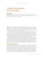
sets of results are shown in Figure 1.
Even more recently (January 2001) a survey by Risk Magazine has estimated the
size of the credit derivatives market at year-end 2000 to be around $810 billion.
This number was determined by polling dealers who were estimated to account
for about 80% of the total market.
All of these reports show that the size of the credit derivatives market has increased
at a phenomenal pace, with an annual growth rate of over 50%. It is estimated by
the BBA survey that the market will achieve a size close to $1.5 trillion by the end
of 2001. To put this into context, the total size of all outstanding dollar denominated
corporate, utility, and financial sector bond issues is around $4 trillion.

Figure 1. Total Outstanding Notional of the Credit Derivatives Market,
1997-2000
0
200
400
600
800
1,000
1997 1998 1999 2000
$ billions
BBA
OCC
The growth of the credit derivatives
market has been recognised by a
number of different surveys.
A market size close to $1.5 trillion is
predicted for the end of 2001.
STRUCTURED CREDIT RESEARCH
7
Lehman Brothers International (Europe), March 2001
2.2 Market Breadth
In terms of the credits actively traded, the credit derivative market spans across
banks, corporates, high-grade sovereign and emerging market sovereign debt.
Recent estimates show corporates accounting for just over 50% of the market,
with the remainder split roughly equally between banks and sovereign credits.
The 2001 survey by Risk Magazine provides a more detailed geographical break-
down. It reported that 41% of default swaps are linked to U.S. credits, 38% to
European credits, 13% to Asian, and 8% to non-Asian emerging markets.
A 1998 survey by Prebon Yamane of all transactions carried out in 1997 reported that
93% of those referenced to Asian issuers were to sovereigns. In contrast, 60% of

those referenced to U.S. issuers were to corporates, with the remainder split between
banks (30%) and sovereigns (10%). Those referenced to European issuers were more
evenly split, with sovereigns accounting for 45%, banks 29%, and corporates 26%.
Clearly, the credit derivative market is not restricted to any one subset of the
credit markets. Indeed, it is the ability of the credit derivative market to do any-
thing the cash market can do and potentially more that is one of its key strengths.
For example, it is possible to structure credit derivatives linked to the credit qual-
ity of companies with no tradable debt. Companies with exposure to such credits
can use this flexibility to hedge their exposures, while investors can diversify by
taking exposure to new credits that do not exist in a cash format.
2.3 Participants
The wide variety of applications of credit derivatives attracts a broad range of
market participants. Historically, banks have dominated the market as the biggest
hedgers, buyers, and traders of credit risk. Over time, we are finding that other
types of player are entering the market. This observation was echoed by the re-
sults of the BBA survey, which produced a breakdown of the market by the type
of participant. The results are shown in Figure 2.
The market encompasses corporate
and sovereign credits.
U.S., European, and Asian-linked
credit derivatives are all traded.
Banks continue to dominate the
credit derivatives market.
Figure 2. A Breakdown of Who Buys and Sells Protection by Market Share
at the Start of 2000.
Counterparty Protection Protection
Buyer (%) Seller (%)
Banks 63 47
Securities Firms 18 16
Insurance Companies 7 23

Corporations 6 3
Hedge Funds 3 5
Mutual Funds 1 2
Pension Funds 1 3
Government/Export Credit Agencies 1 1
Source: British Bankers’ Association Credit Derivatives Report 2000.
STRUCTURED CREDIT RESEARCH
Lehman Brothers International (Europe), March 2001
8
As in its earlier 1998 survey, the BBA found that banks easily dominate the credit
derivatives market as both buyers and sellers of credit protection. Since banks are
in the business of lending and thereby taking on credit exposure to borrowers, it
is not surprising that they use the credit derivatives market to buy credit protec-
tion to reduce their exposure.
Though the precise details may vary between different regulatory jurisdic-
tions, banks can use credit derivatives to offset and reduce regulatory capital
requirements. On a single asset level, this may be achieved using a standard
default swap. More commonly, banks are now using credit derivatives to
securitize whole portfolios of bonds and loans. This technology, known as the
synthetic CLO and explained in detail in Section 5.8, can be used by banks
with the purpose of reducing regulatory capital, reducing credit risk concen-
trations, and enhancing return on capital. Indeed, the 2001 Risk Magazine
survey finds that banks as counterparties in synthetic securitisations account
for 18% of the market.
At the same time, banks are also seeking to maximize return on equity, and credit
derivatives provide an unfunded way for banks to earn yield from their under-
used credit lines and to diversify concentrations of credit risk. As a consequence,
we see that banks are the largest sellers of credit protection.
Securities firms are the second-most dominant player in the market. With their
market making and risk-taking activities, securities firms are a major provider of

liquidity to the market. As they tend to run a flat trading book, we see that they
are buyers and sellers of protection in approximately equal proportions.
An interesting development in the credit derivatives market has been the in-
creased activity of insurance and re-insurance companies, on both the asset and
liability side. For insurance companies, selling protection using credit deriva-
tives presents a new asset class that can be used to earn income and diversify
revenue away from their core business of insurance. The credit derivatives market
is ideal for this since through the structuring of second loss products, it creates
the very highly rated securities that insurance companies require in order to
maintain their high ratings. As compensation for their novelty and lower liquid-
ity compared with Treasury bonds, these securities can return a substantially
higher yield for a similar credit rating. On the liability side, re-insurance com-
panies are also prepared to take leveraged credit risks, such as retaining the
most subordinate piece on tranched credit portfolios. This is seen as just an-
other way to write insurance contracts.
As protection buyers, this growth in usage by insurance companies has been
driven by their desire to hedge various insurance risks. For instance, in the
area of insuring project financing within developing economies, the sover-
eign credit derivatives market provides a good, though imperfect, hedge against
any sovereign risk to which they may be exposed. Re-insurance companies
who typically develop concentrations of credit risk can use credit derivatives
Credit derivatives can be used by
banks to reduce regulatory capital.
For banks, credit derivatives present
an unfunded way to diversify
revenue.
Insurance and re-insurance compa-
nies have become major players in
the credit derivatives market.
STRUCTURED CREDIT RESEARCH

9
Lehman Brothers International (Europe), March 2001
Figure 3. Market Share of Outstanding Notional for Credit Derivative
Products
Market Share
Credit Derivative Instrument Type (% Notional) at End 1999
Credit Default Products 38%
Portfolio/CLOs 18%
Asset Swaps 12%
Total Return swaps 11%
Credit Linked Notes 10%
Baskets 6%
Credit Spread products 5%
Source: British Bankers’ Association Credit Derivatives Report 2000.
to reduce this exposure and so enable them to take on new more diversified
business without an overall increase in risk. Over the next few years, we ex-
pect to see re-insurance companies account for an even larger share of the
credit derivatives market.
Hedge funds are another growing particpant. Some focus on exploiting the arbi-
trage opportunities that can arise between the cash and default swap markets.
Others focus on portfolio trades such as investing in CDOs. Equity hedge funds
are especially involved in the callable asset swap market in which convertible
bonds have their equity and credit components stripped. These all add risk-taking
capacity and so add to market liquidity.
2.4 Products
There are a number of different products that may be classified as credit deriva-
tives, ranging from the simple asset swap to the synthetic CLO. Figure 3 shows
the market share (as a percent of market notional) of the different credit deriva-
tive instruments as reported by the BBA for the start of 2000.
Dominating the market, credit default products—default swaps—account for

more than twice as much of the market as the second-most popular product. In
practice, default swaps have become the de facto unfunded credit derivative
instrument, with credit spread options and similar spread driven products pushed
down into last place.
The growth in usage of synthetic CLOs that have an embedded portfolio default
swap has been very sudden—they did not even appear in the previous (1997-
1998) BBA survey. Part of their prominence is attributable to the fact that a typical
CLO portfolio default swap has a notional size of $2-$5 billion. This compares
with the typical default swap trade, which has a notional of $10-$50 million.
Equity hedge funds are active
participants in the convertible asset
swap market.
Default swaps dominate the credit
derivatives market.
STRUCTURED CREDIT RESEARCH
Lehman Brothers International (Europe), March 2001
10
Another new entrant is the default basket. This is also a portfolio credit product
that introduces a new way for investors to leverage their credit risk and earn
yield. Though it constitutes only 6% of the outstanding market notional, we ex-
pect this percentage to increase over the next few years. The default basket is
unique in the sense that it is the simplest credit derivative that allows investors to
trade default correlation.
As these results have shown, the credit derivative market has evolved rapidly
over the last five years in terms of increasing its size, broadening its base of
participants, and expanding its list of products. We believe that the market has
achieved critical mass and has become the most effective and efficient way to
commoditize credit risk. The market is also converging rapidly towards
standardised products, especially for the credit default swap. With the increased
participation of the newer players such as insurance, re-insurance companies,

and hedge funds, we expect further evolution and growth and increased liquidity
in the credit derivatives market.
Portfolio default swap trades are
much fewer in number, but are done
in a very large size.
The credit derivatives market has
achieved critical mass.
STRUCTURED CREDIT RESEARCH
11
Lehman Brothers International (Europe), March 2001
3. CREDIT RISK FRAMEWORK
3.1 Probability of Default and Recovery
The commoditization and transfer of credit risk has been one of the major achieve-
ments of the credit derivatives market. However, to be able to do this, we need a
framework for valuing credit risk. It is clear that the compensation that an inves-
tor receives for assuming a credit risk and the premium that a hedger would need
to pay to remove a credit risk must be linked to the size of the credit risk. This can
be defined in terms of:
1) The likelihood of default
2) The size of the payoff or loss following default.
The best example is a one-year zero coupon defaultable bond. Let us assume that
the probability that the bond will default over the next year is p. If the bond does
default, we assume that it pays a recovery rate R, which is a fixed percentage of
the face value. We further assume that this recovery is paid at the maturity date of
the bond. One can model this as a simple single-period binomial tree, as shown in
Figure 4, where the price of the bond, P
Risky,
is the expected payoff discounted off
the risk-free curve. This gives:
()

100)1(100
1
1
×−+××
+
= pRp
r
P
Risky
where r is the one-year risk-free rate. Note that the market uses the LIBOR swap
curve as the risk-neutral default-free interest rate, since that is the level at which
most market participants fund their hedges.
Figure 4. Simple One-Period Model of Default That Pays Recovery at
Maturity

Bond redeems at
par $100
Bond pays
a

recovery amoun
t

$100×R
Bond defaults with
probability p
Bond survives wit
h

probability 1-p

P
Risky
To price credit risk, we need to have
a quantitative framework.
STRUCTURED CREDIT RESEARCH
Lehman Brothers International (Europe), March 2001
12
If the one-year probability of default is 0.75%, the recovery rate is assumed to be
50%, and the one-year risk-free rate is 5%, the price of the bond is given by

()
88.94$1009925.050.01000075.0
05.1
1
=×+××=
Risky
P
which is clearly lower than the risk-free zero coupon bond price:
24.95$
05.1
100
==
−FreeRisk
P
.
For a zero coupon bond, we define the credit quality using the spread s as fol-
lows:
)1)(1(
100
sr

P
Risky
++
=
.
Using the above example, we find that s = 37.7 bp.
It is possible to show that one can accurately approximate the credit spread using
the credit triangle formula, shown in Figure 5, which states that the annualized
compensation for assuming a credit risk, the credit spread, S, is equal to the prob-
ability of default (per annum), P, times the loss in the event of a default. For a par
asset, the loss is par minus the recovery rate R. We call this equation the credit
triangle because it has three unknowns, and we can solve for any one provided
we know the other two.
If we substitute the probability of default and assumed recovery rate from the
above example into the credit triangle equation, we find that
bps 5.37)5.01(0075.0 =−×≈
.
The credit spread equals the default
probability times the loss in the
event of a default.
Figure 5. The Credit Triangle
S
PR
)1( RPS −=
STRUCTURED CREDIT RESEARCH
13
Lehman Brothers International (Europe), March 2001
There is considerable variation in
the recovery rate for bonds
of the same seniority.

The credit triangle can be used to
examine relative value within the
capital structure.
And we see that this “rule-of-thumb” is very accurate (correct to 0.2 bp). This
is a simple, yet very powerful formula for analysing credit spreads and what
they imply about default probabilities and recovery rates, and vice-versa.
Within the credit derivatives market, understanding such a relationship is es-
sential when thinking about how to price instruments such as fixed recovery
default swaps.
It is also a very useful formula for examining relative value within the capital
structure of a company. Since cross default provisions mean that it is almost
always the case that all of the debt of a company defaults together, the only
thing that differentiates between senior and subordinated debt is the expected
recovery in the event of default. All of the company’s bonds, therefore, have
the same default probability. Using this fact, one can use the Credit Triangle
to derive an equation expressing the subordinated “fair-value” spread as a
function of the senior spread and the respective recovery rates of the senior
and subordinated bonds.
SENIOR
SENIOR
SUB
SUB
S
R
R
S ×
−
−
=
)1(

)1(
For example, if R
SENIOR
= 50%, R
SUB
= 20% and the senior LIBOR spread S
SENIOR
=
50 bp, this implies that the subordinate spread should be 80 bp. One should qualify
this result by noting that the LIBOR spread of a security may contain other fac-
tors such as liquidity and credit risk premia. Nevertheless, this simple relationship
does provide a useful starting point for analysing relative value.
3.2 Empirical Studies of Recovery Rates
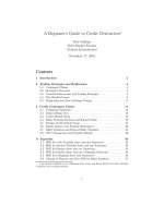
The market standard source for recovery rates is Moody’s historical default rate
study (see www.moodysqra.com), the results of which are plotted in Figure 6. It
shows how the recovery rate of a defaulted asset depends on the level of subordi-
nation. By plotting the first and third quartiles, it is clear that there is a very wide
variation in the recovery rate, even for the same level of seniority.
These results are based on U.S. corporate defaults and so do not take into account
the variations in bankruptcy laws that exist between different countries. Note
that these recovery rates are not the actual amounts received by the bondholders
following the workout process. Instead, they represent the price of the defaulted
asset as a fraction of par some 30 days after the default event.
3.3 Empirical Studies of Default Probabilities
Figure 7 shows Moody’s cumulative default probabilities by rating and maturity.
These are the average probability of a bond that starts in the given rating default-
ing within the time horizon given. Clearly, we see that highly rated bonds have a
lower cumulative default probability than lower-rated bonds.
Using the credit triangle, it is possible to imply out an implied cumulative default
probability from market spreads. Typically, one finds that this default probability is

STRUCTURED CREDIT RESEARCH
Lehman Brothers International (Europe), March 2001
14
Market implied default probabilities
are typically higher than historical
default probabilities.
Credit curve shapes contain
information about market
expectations for the credit.
greater than that implied by empirical analysis. There are a number of reasons why
this is the case. First, the credit spread of a bond will usually contain a liquidity
component. After all, no bond is as liquid as a Treasury bond or a LIBOR swap.
Then, there may be a component to account for regulatory capital effects. There
will be a credit risk premium designed to protect the bond holder against changes in
the credit quality of the issuer. Finally, market spreads are forward looking and
asset specific, whereas the numbers in Figure 7 are based on historical defaults and
are averaged over a large number of bonds within each rating class.
3.4 Credit Curves
Investors have different views about how the credit risk of a company will
change over time. This is manifested in the shape of the credit curve: the excess
yield over some benchmark interest rate of a credit as a function of the maturity
of the credit exposure.
This excess yield, known as a credit spread, can be expressed in a variety of
ways, including the asset swap spread, the default swap spread, the par floater
Cumulative Default Probability to Year (%)
Rating 1 2345 6 78910
Aaa 0.00 0.00 0.00 0.04 0.12 0.21 0.31 0.42 0.54 0.67
Aa 0.02 0.04 0.08 0.20 0.31 0.43 0.55 0.67 0.76 0.83
A 0.01 0.05 0.18 0.31 0.45 0.61 0.78 0.96 1.18 1.43
Baa 0.14 0.44 0.83 1.34 1.82 2.33 2.86 3.39 3.97 4.56

Ba 1.27 3.57 6.11 8.65 11.23 13.50 15.32 17.21 19.00 20.76
B 6.16 12.90 18.76 23.50 27.92 31.89 35.55 38.69 41.51 44.57
Figure 7. Moody’s Cumulative Default Probabilities by Letter Rating from 1-10 years, 1970-2000.
0 102030405060708090100
Senior/Secured Bank Loans
Equipment Trust Bonds
Senior/Secured Bonds
Senior/Unsecured Bonds
Senior/Subordinated Bonds
Subordinated Bonds
Junior/Subordinated Bonds
Preferred Stocks
Recovery Price as % of Par Amount
Figure 6. Moody’s Historical Recovery Rate Distributions, 1970-1999, for
Different Levels of Subordination. Each Bar Starts at the 1
st
Quartile Then Changes Color at the Average and Ends at the 3
rd
Quartile.
Source : Moody’s Investors Services.
STRUCTURED CREDIT RESEARCH
15
Lehman Brothers International (Europe), March 2001
spread, and the option-adjusted or zero-volatility spread. The exact significance
of these spreads will be defined in forthcoming sections. There are three main
credit curve shapes, which are shown in Figure 8:
Upward Sloping: Most credits exhibit an upward sloping credit curve. This can be
explained as expressing the view that within the short term, the quality of the credit
is expected to remain constant. However, the further into the future we look, the less
we can be certain that the credit will not deteriorate. The credit spread increases in

order to compensate the investor for this increased uncertainty.
Humped: This shape is commonly observed for credits that are viewed as likely
to worsen in the medium term—the chance of defaulting in the very short term is
low. As the maturity increases, the credit spread then falls to reflect the view that
should the credit survive the medium term, it will be more likely to survive the
long term.
Downward Sloping (Inverted): The inverted curve is usually associated with
credits that have experienced a significant deterioration to the extent that a de-
fault is probable. The bonds begin to trade on a price basis —bonds of the same
seniority trade with the same price irrespective of their maturity and coupon. This
has the effect of elevating short-maturity spreads and inverting the spread curve.
3.5 Credit Spreads
There are a number of different measures of credit spread used in the credit mar-
kets. These may be real spreads associated with specific types of instrument or
may be measures of excess yield. However, these different credit spreads may
include effects other than pure credit risk. For example, Treasury credit spreads,
There are many different measures
of credit spread, each with its
own properties
Figure 8. The Three Main Credit Spread Curve Shapes.
0
100
200
300
400
500
600
700
0 5 10 15 20 25 30
Maturity

Credit Spread (bp
)
Upward
Humped
Inverted
STRUCTURED CREDIT RESEARCH
Lehman Brothers International (Europe), March 2001
16
which measure credit risk versus the Treasury yield curve, may include effects of
liquidity, coupon size, risk premia, and the supply and demand for Treasury bonds.
We summarise the main spread types in Figure 9.
Figure 9. Different Credit Spreads
Spread Type Definition Comment
Yield Spread
Par Floater Spread
Asset Swap Spread
Default Swap Spread
Discount Margin
Option Adjusted Spread
(Zero Volatility Spread)
Difference between the yield of the bond
and the benchmark Treasury yield.
Spread over LIBOR paid by a floater
issued today which prices to par.
Spread over LIBOR received by an
asset swap buyer who swaps the fixed
coupon of a fixed rate bond to floating
for an up front cost of par.
The amortised premium for a contract
that pays par minus recovery on an

asset which defaults and nothing
otherwise.
The flat yield spread required to reprice
a floating rate bond to par.
The flat continuously compounded
spread to the LIBOR zero rate which
reprices the bond.
This is a spread to the Treasury curve so contains the swap
spread. It is a measurement of the yield of a position
consisting of long corporate and short the benchmark
Treasury benchmark. May also involve a maturity differ-
ence between risky bond and benchmark Treasury.
See section 4.1.
If the underlying asset is valued at par, this equals the par
floater spread. If the asset trades away from par, the asset
swap spread also contains coupon-linked effects. Bonds
with the same issuer, same seniority and same maturity but
different coupons will have different asset swap spreads.
See section 4.2.2 for discussion and section 8.3 for
calculation details.
Ignoring funding and repo effects, the default swap is
economically equivalent to a par floater and so should have
the same spread. See Section 4.3 for details.
Calculation (see Section 8.2) ignores the shape of the
LIBOR curve. Equals the Par Floater Spread for a bond
trading at par.
Historically used to value the embedded issuer option in
callable bonds but can also be used to quantify the effect
of credit. Also known as the Zero Volatility Spread, this is
a continuously compounded version of the par floater

spread. A good measure of the excess yield due to credit.
(see Section 8.4 for calculation details).
STRUCTURED CREDIT RESEARCH
17
Lehman Brothers International (Europe), March 2001
4. SINGLE-NAME CREDIT DERIVATIVE PRODUCTS
We begin this section with an instrument that is definitely not a credit derivative:
the floating-rate note. Its inclusion is due to its importance as an instrument whose
pricing is driven almost exclusively by credit. As such, it serves as a benchmark
for much of credit derivative pricing, and no discussion of credit derivatives is
complete without it.
4.1 Floating-Rate Notes
4.1.1 Description
A floating-rate note (FRN) is a bond that pays a coupon linked to a variable
interest rate index. As we shall describe below, this has the effect of eliminating
most of the interest rate sensitivity of the note, making it almost a pure credit
play. As a result, the price action of a floating-rate note is driven mostly by the
changes in the market-perceived credit quality of the note issuer.
In many cases, the variable interest rate index used is the London Interbank Of-
fered Rate - LIBOR. In continental Europe, the euro benchmark is called Euribor
or Eibor. Although calculated slightly differently, all of these indices are a mea-
sure of the rate at which highly rated commercial banks can borrow. They therefore
reflect the credit quality of the (roughly) AA-rated commercial banking sector.
While the senior short-term floaters of AA-rated banks pay a coupon close to
LIBOR flat and trade at a price close to par, in the credit markets, many floaters
are issued by corporates with much lower credit ratings. Also, many AA-rated
banks issue floating-rate notes that are subordinate in the capital structure. In
either case, investors require a higher yield to compensate them for the increased
credit risk. At the same time, the coupons of the bond must be discounted at a
higher interest rate than LIBOR to take into account this higher credit risk.

Therefore, in order to issue the note at (or slightly below) par, the coupon on the
floating-rate note must be set at a fixed spread over LIBOR. In fact, it is easy to
show that this fixed spread, S, must be set equal to the spread over LIBOR at
which the cash flows of the issuer are discounted (see Section 8.1 for details).
This spread is known as the par floater spread, F. The par floater spread can be
thought of as a measure of the market-perceived credit risk of the note issuer. The
fixed spread of a floating-rate note therefore tells us the par floater spread and,
hence, the credit quality of its issuer when it was issued at par.
In Figure 10, we show the cash flows for an example 3-year floating-rate note
whose coupon resets and pays every six months—the variable rate is therefore 6-
month LIBOR plus a fixed spread of 104bp (52bp semi-annually).
4.1.2 Pricing Aspects
Floating-rate notes have a much lower interest rate sensitivity than fixed-rate
bonds. If LIBOR interest rates increase, the resulting increase in the implied fu-
ture LIBOR coupons is almost exactly offset by the increase in the rate at which
Floating-rate notes have a very low
interest rate sensitivity.
The interest rate sensitivity is higher
between coupon dates.
LIBOR is the most commonly used
benchmark variable interest rate
index.
STRUCTURED CREDIT RESEARCH
Lehman Brothers International (Europe), March 2001
18
they are discounted. Similarly, when LIBOR falls, the implied future coupons
decrease in value, but this is offset as they are discounted back to today at a lower
rate of interest. As a result, the interest rate sensitivity of a floating rate note is
much less than that of a fixed-rate bond of the same maturity.
On coupon dates, whether the price of a floating rate note is above or below par is

determined solely by its par floater spread. If this is greater than the fixed spread
paid by the floater, then it will trade below par. If the par floater spread is lower
than the fixed spread, the floating rate note will trade above par. How far above or
below par is determined by the note’s maturity, coupon, par floater spread and the
LIBOR curve. This is shown mathematically in Section 8.1.
Between coupon dates, the price of the floating rate note can deviate from par as
a consequence of movements in LIBOR. As the LIBOR component of the next
coupon has been fixed in advance, the value of the next coupon payment is known
today. However we present-value it at a rate of LIBOR plus a spread. This rate
changes as LIBOR changes, so we are exposed to interest rates. This exposure is
known as reset risk. It is usually small, declining to zero as the next coupon is
approached. Provided the par floater spread of the issuer does not change, the
bond should always reprice to par on coupon payment dates.
If the credit curve of the note’s issuer is upward sloping, the par floater spread
will fall as the note approaches maturity. This will cause the bond to increase in
price, as the fixed spread paid will remain unchanged but the note will be dis-
counted at a lower par floater spread. Despite this, as the bond approaches maturity,
the price will revert to par.
In addition to the par floater spread, another convention for quoting the credit spread
of an FRN is to use the discount margin. This is a very similar idea to the par
floater spread but is defined slightly differently. It is based on a calculation that
The discount margin is a commonly
used measure of the credit spread for
floating rate notes.
Figure 10. The Cash Flows of a 3-Year Floating-Rate Note.
100
100
Floating coupons of Libor plus
52bp paid semi-annually
FRN Issued at par

6M 24M18M12M 36M30M
STRUCTURED CREDIT RESEARCH
19
Lehman Brothers International (Europe), March 2001
assumes a flat LIBOR curve and so does not take into account the shape of the term
structure of the LIBOR curve on the present-valuing of future cash flows. We de-
scribe this in more detail in Section 8.1.2. In practice, the difference between the
LIBOR spread and the par floater spread is very small, but not small enough to
ignore. It also means that the discount margin calculation differs from the approach
used in pricing credit derivatives that use the full shape of the LIBOR curve.
4.1.3 Applications
A large proportion of the floating-rate note market is issued by banks to satisfy
their bank capital requirements and may be fixed maturity or perpetual. Tradi-
tionally, perpetual bonds have consituted a sizeable portion of the floating rate
note market. The advantage of a floating rate perpetual is that it has a low interest
rate duration despite having an infinite maturity.
In addition to banks, a large number of corporate and emerging market bonds are
issued in floating rate format. For example, some Brady bonds such as the Argen-
tina FRBs of ’05 pay a coupon of LIBOR plus 13/16ths.
In summary, floating rate notes are a way for a credit investor to buy a bond and
take exposure to a credit without taking exposure to interest rate movements.
This makes it possible for credit investors to focus on their speciality—under-
standing and taking a view about the credit quality of the issuer. However, most
bonds are fixed rate and so incorporate a significant interest rate sensitivity. To
turn them into pure credit plays, we need to use the asset swap.
4.2 Asset Swaps
4.2.1 Description
An asset swap is a synthetic floating-rate note. By this we mean that it is a spe-
cially created package that enables an investor to buy a fixed-rate bond and then
hedge out almost all of the interest rate risk by swapping the fixed payments to

floating. The investor takes on a credit risk that is economically equivalent to
buying a floating-rate note issued by the issuer of the fixed-rate bond. For assum-
ing this credit risk, the investor earns a corresponding excess spread known as the
asset swap spread.
While the interest rate swap market was born in the 1980s, the asset swap mar-
ket was born in the early 1990s. It continues to be most widely used by banks,
which use asset swaps to convert their long-term fixed-rate assets, typically
balance sheet loans and bonds, to floating rate in order to match their short term
liabilities, i.e., depositor accounts. During the mid-1990s, there was also a sig-
nificant amount of asset swapping of government debt, especially Italian
Government Bonds.
The most recent BBA survey has estimated the size of the asset swap market to be
about 12% of the total credit derivatives market, implying an outstanding no-
tional on the order of $100 billion. This is believed to be a lower limit, as many
institutions do not formally classify asset swaps as credit derivatives. This is a
Floating-rate notes enable the
investor to take a pure credit view.
Asset swaps convert a fixed-rate
bond into a pure credit play.
STRUCTURED CREDIT RESEARCH
Lehman Brothers International (Europe), March 2001
20
debatable point. However, what is well accepted is the fact that asset swaps are a
key structure within the credit markets and are widely used as a reference for
credit derivative pricing.
There are several variations on the asset swap structure, with the most widely traded
being the par asset swap. In its simplest form, it can be treated as consisting of two
separate trades. In return for an up-front payment of par, the asset swap buyer:
 Receives a fixed rate bond from the asset swap seller. Typically the bond is
trading away from par.

 Enters into an interest rate swap to pay to the asset swap seller a fixed coupon
equal to that of the asset. In return, the asset swap buyer receives regular
floating rate payments of LIBOR plus (or minus) an agreed fixed spread.
The maturity of this swap is the same as the maturity of the asset.
The transaction is shown in Figure 11. The fixed spread to LIBOR paid by the
asset swap seller is known as the asset swap spread and is set at a breakeven value
such that the net present value of the transaction is zero at inception.
In Figure 12, we show the cash flows for an example asset swap of a bond that
has a maturity date of 20 May 2003 and an annual coupon of 5.625% and is
trading at a price of 101.70. The frequency on the floating side is semi-annual.
The breakeven value of the asset swap spread makes the net present value of all
of the cash flows equal to par, the up-front price of the asset swap.
4.2.1 Pricing Aspects
The most important thing to understand about an asset swap is that the asset swap
buyer takes on the credit risk of the bond. If the bond defaults, the asset swap buyer
Figure 11. Mechanics of a Par Asset Swap
Asset Swap
Seller
Asset Swap
Buyer
Bond
C
C
LIBOR + S
At initiation Asset Swap buyer purchases bond worth full price P in return for par
and enters into an interest rate swap paying a fixed coupon of C in return for LIBOR plus asset swap spread S
If default occurs the asset swap buyer loses the coupon and principal redemption on the bond. The
interest rate swap will continue until bond maturity or can be closed out at market value.
Asset Swap
Seller

Asset Swap
Buyer
Bond
C
C
LIBOR + S
Bond
worth P
100
Asset Swap
Seller
Asset Swap
Buyer
It is the combination of the purchase
of an asset and the entry into an
interest rate swap.
STRUCTURED CREDIT RESEARCH
21
Lehman Brothers International (Europe), March 2001
has to continue paying the fixed side on the interest rate swap that can no longer be
funded with the coupons from the bond. The asset swap buyer also loses the
redemption of the bond that was due to be paid at maturity and is compensated with
whatever recovery rate is paid by the issuer. As a result, the asset swap buyer has a
default contingent exposure to the mark-to-market on the interest rate swap and to
the redemption on the asset. In economic terms, the purpose of the asset swap spread
is to compensate the asset swap buyer for taking on these risks.
For most corporate and emerging market credits, the asset swap spread will be
positive. However, since the asset swap spread is quoted as a spread to LIBOR,
which is a reflection of the credit quality of AA-rated banks, for higher-rated
assets the asset swap spread may actually be negative.

In Figure 13, we demonstrate an example of the default contingent risk assumed
by the asset swap buyer. In the example, the bond is trading at $90. Assume that
we are at the moment just after trade inception so that the value of the swap has
not changed. If the bond defaults with $40 recovery price, the asset swap buyer
loses $60, having just paid par to buy a bond now worth $40. However, he/she
is also payer of fixed in a swap that is 10 points in his/her favor. The net loss is
therefore $50, the difference between the full price of the bond and the recov-
ery price.
However, consider what happens if the bond has a high coupon and so is trading
20 points above par. This is shown in Figure 14. This time, if the bond defaults
immediately with a recovery price of $10, the asset swap buyer will have lost a
The asset swap buyer takes on the
credit risk of the fixed rate bond.
Figure 12. Cash Flows for 3-Year Tecnost Par Asset Swap Trade
5.625%
101.70
100.00
5.625%
5.625%
L+52bp
L+52bp
L+52bp L+52bp L+52bp L+52bp
Fixed coupons paid annually to the asset swap seller
Floating coupons paid semi-annually to the asset swap buyer
Initial exchange
No exchange at
maturity
Dec00 Ma
y
01

Dec01
May02
Dec02
May03
Figure 13. Asset Swap on a Discount Bond
Bond Swap Total
Value At Inception +$90 +$10 +$100
Value Following Default +$40 +$10 +$50
Loss -$50 $0 -$50
The asset swap buyer has a default
contingent exposure to the mark-to-
market on the interest rate swap.
STRUCTURED CREDIT RESEARCH
Lehman Brothers International (Europe), March 2001
22
total of $110: the asset swap buyer paid par for a bond now worth $10 and is party
to a swap which has a negative mark-to-market of 20 points. As a result, the
investor has actually leveraged the credit exposure and can, therefore, lose more
than the initial investment. However, he/she is compensated for this with a higher
asset swap spread.
For a par bond, the maximum loss the asset swap buyer can incur is par minus the
recovery price. In terms of expected loss, this makes an asset swap similar to a
par floater since the expected loss on a floater that trades at par is also par minus
recovery. However, in actual practice, this comparison is mostly academic since
there will be wide differences between these spreads due to liquidity, market size,
funding costs, supply and demand, and counterparty risk.
As time passes and interest rates and credit spreads change, the mark-to-market on
the asset swap will change. To best understand the LIBOR and credit spread sensitiv-
ity of the asset swap from the perspective of the asset swap buyer, we use the PV01,
defined as the change in price for a one basis point upward shift in the par curve.

For example, consider a 10-year bond with a par floater spread of 50 bp and an
annual coupon of 6.0%. As the bond is trading close to par, it will have an asset
swap spread of about 50 bp. Using a LIBOR curve from October 1999, the PV01
sensitivities are calculated as shown in Figure 15.
The net PV01 is much smaller than that of the fixed-rate bond. While a fixed rate
bond will change in price by about 7.5 cents for a one-basis-point change in
interest rates, the asset swap will change in price by only 0.17 cents, a reduction
in interest rate sensitivity by a factor of about 44.
The key point here is that the sensitivity of the bond price to parallel movements
in the yield curve will be less than the sensitivity of the fixed side of the swap to
parallel shifts in the LIBOR curve. This is true only provided the issuer curve is
above the LIBOR curve, which is typically the case. The asset swap buyer, there-
Figure 15. PV01 Sensitivities of an Asset Swap
Leg PV01
Fixed Rate Bond -7.540
Swap +7.710
Net +0.170
The asset swap buyer can leverage
credit exposure.
Figure 14. Asset Swap on a Premium Bond
Bond Swap Total
Value At Inception +$120 -$20 +$100
Value Following Default +$10 -$20 -$10
Loss -$110 $0 -$110
STRUCTURED CREDIT RESEARCH
23
Lehman Brothers International (Europe), March 2001
fore, has a very small residual exposure to interest rate movements, which only
becomes apparent when LIBOR spreads widen significantly.
While the sensitivity to changes in LIBOR swap rates is almost negligible (unless

LIBOR spreads are very wide), the sensitivity to changes in the LIBOR spread is
equivalent to being long the bond. This echoes the claim that an asset swap trans-
forms a fixed-rate bond into a pure credit play.
An important consideration in par asset swaps is counterparty default risk. Pay-
ing par to buy a bond that is trading at a discount results in the asset swap buyer’s
having an immediate exposure to the asset swap seller equal to par minus the
bond price. The opposite is true when the bond is trading at a premium to par. The
size of this counterparty exposure can change over time as markets move. How-
ever these exposures can be mitigated or reversed using other variations of the
standard par asset swap. Equally, one could use other traditional methods such as
collateral posting, netting, and credit triggers.
4.2.2 Calculating the Asset Swap Spread
The breakeven asset swap spread A is computed by setting the net present value of all
cash flows equal to zero. When discounting cash flows in the swap, we use the LIBOR
curve, implying that the parties to the swap have the same credit quality as AA-rated
bank counterparties. It is shown in Section 8.3 that the asset swap spread is given by
01PV
PP
A
MARKETLIBOR
−
=
where we define P
LIBOR
to be the present value of the bond priced off the LIBOR
swap curve, P
MARKET
is the actual full market price of the bond, and PV01 is the
present value of a one-basis-point annuity with the maturity of the bond, present
valued on the LIBOR curve.

On a technical note, when the asset swap is initiated between coupon dates, the
asset swap buyer does not pay the accrued interest explicitly. Effectively, the full
price of the bond is at par. At the next coupon period, the asset swap buyer re-
ceives the full coupon on the bond and, likewise, pays the full coupon on the
swap. However, the floating side payment, which may have a different frequency
and accrual basis to the fixed side, is adjusted by the corresponding accrual fac-
tor. Therefore, if we are exactly halfway between floating side coupons, the floating
payment received is half of the LIBOR plus asset swap spread. This feature pre-
vents the calculated asset swap spread from jumping as we move forward in time
through coupon dates.
4.2.3 Applications
The main reason for doing an asset swap is to enable a credit investor to take
exposure to the credit quality of a fixed-rate bond without having to take interest
rate risk. For banks, this has enabled them to match their assets to their liabilities.
As such, they are a useful tool for banks, which are mostly floating rate based.
The interest rate sensitivity of an
asset swap is very small.
Counterparty risk can be factored
into the pricing or reduced using
collateral.
STRUCTURED CREDIT RESEARCH
Lehman Brothers International (Europe), March 2001
24
Asset swaps can be used to take advantage of mispricings in the floating rate note
market. Tax and accounting reasons may also make it advantageous for investors
to buy and sell non-par assets at par through an asset swap.
Using forward asset swaps, it is possible to go long a credit at some future date
at a spread fixed today. If the bond defaults before the forward date is reached,
the forward asset swap trade terminates at no cost. The investor does not take on
the default risk until the forward date. Since credit curves are generally upward

sloping, a forward asset swap can often make it cheaper for an investor to go long
a credit on a forward basis than to buy the credit today.
Another variation is the cross-currency asset swap. This enables investors to
buy a bond denominated in a foreign currency, paying for it in their base cur-
rency, pay on the swap in the foreign currency, and receive the floating-rate
payments in their base currency. The cash flows are converted at some predefined
exchange rate. In this case, there is an exchange of principal at the end of the
swap. This structure enables the investors to gain exposure to a foreign currency
denominated credit with minimal interest rate and currency risk provided the
asset does not default. However, for assets with very wide spreads, these residual
risks can be material.
For callable bonds, where the bond issuer has the right to call back the bond at a
pre-specified price, asset swap buyers will need to be hedged against any loss on
the swap since they will no longer be receiving the coupon from the asset. In this
case, the asset swap buyers will want to be able to cancel the swap on any of the call
dates by buying a Bermudan-style receiver swaption. This package is known as a
cancellable asset swap. Most U.S. agency callable bonds are swapped in this way.
Callable asset swaps may also be used to strip out the credit and equity components
of convertible bonds. The investor buys the convertible bond on asset swap from the
asset swap seller and receives a floating rate coupon consisting of LIBOR plus a
spread. The embedded equity call option is also sold separately to an equity investor.
So that the equity conversion option can be exercised, the asset swap must be callable
by the asset swap seller with a strike set at some fixed spread to LIBOR. This enables
the asset swap seller to retrieve the convertible bond and convert it into the underly-
ing stock in the event that the equity option holder wishes to exercise.
This example demonstrates how credit derivatives make it possible to split up a
hybrid product such as a convertible bond, which has limited demand, into new
exposures that better match the differing specialities and risk appetities of inves-
tors. Typically, fixed-income investors will be able to earn a higher yield from the
stripped asset swap than otherwise available in the conventional bond market.

Equity investors may be able to buy the conversion option more cheaply (at a
lower implied volatility) than is available in the equity derivatives market.
The asset swap market continues to be a very active over-the-counter market
where most trades can be structured to match the needs of the investor.
There are many applications
for assets swaps.
Callable asset swaps can be used to
strip out the equity and fixed income
components of convertible bonds.