Permitted water pollution discharges and population cancer and non-cancer mortality: toxicity weights and upstream discharge effects in US rural-urban areas doc

RESEARCH Open Access
Permitted water pollution discharges and
population cancer and non-cancer mortality:
toxicity weights and upstream discharge effects
in US rural-urban areas
Michael Hendryx
1,2,4*
, Jamison Conley
1,3
, Evan Fedorko
1,3
, Juhua Luo
1,2
and Matthew Armistead
1
Abstract
Background: The study conducts statistical and spatial analyses to investigate amounts and types of permitted
surface water pollution discharges in relation to population mortality rates for cancer and non-cancer causes
nationwide and by urban-rural setting. Data from the Environmental Protection Agency’s (EPA) Discharge
Monitoring Report (DMR) were used to measure the location, type, and quantity of a selected set of 38 discharge
chemicals for 10,395 facilities across the con tiguous US. Exposures were refined by weighting amounts of chemical
discharges by their estimated toxicity to human health, and by estimating the discharges that occur not only in a
local county, but area-weighted discharges occurring upstream in the same watershed. Centers for Disease Control
and Prevention (CDC) mortality files were used to measure age-adjusted population mortality rates for cancer,
kidney disease, and total non-cancer causes. Analysis included multiple linear regressions to adjust for population
health risk covariates. Spatial analyses were conducted by applying geographically weighted regression to examine
the geographic relationships between releases and mortality.
Results: Greater non-carcinogenic chemical discharge quantities were associated with significantly higher non-
cancer mortality rates, regardless of toxicity weighting or upstream discharge weighting. Cancer mortality was
higher in association with carcinogenic discharges only after applying toxicity weights. Kidney disease mortality
was related to higher non-carcinogenic discharges only when both applying toxicity weights and including

upstream discharges. Effects for kidney mortality and total non-cancer mortality were stronger in rural areas than
urban areas. Spatial results show correlations between non-carcinogenic discharges and cancer mortality for much
of the contiguous United States, suggesting that chemicals not currently recognized as carcinogens may
contribute to cancer mortality risk. The geographically weighted regression results suggest spatial variability in
effects, and also indicate that some rural communities may be impacted by upstream urban discharges.
Conclusions: There is evidence that permitted surface water chemical discharges are related to population
mortality. Toxicity weights and upstream discharges are important for understanding some mortality effects.
Chemicals not currently recognized as carcinogens may nevertheless play a role in contributing to cancer mortality
risk. Spatial models allow for the examination of geographic variability not captured through the regression
models.
Keywords: Age-adjusted mortality, Spatial analysis, Water pollution, Cancer, Kidney disease, Rural-urban differences
* Correspondence:
1
West Virginia Rural Health Research Center, West Virginia University,
Morgantown, USA
Full list of author information is available at the end of the article
Hendryx et al. International Journal of Health Geographics 2012, 11:9
/>INTERNATIONAL JOURNAL
OF HEALTH GEOGRAPHICS
© 2012 Hend ryx et al; licensee BioMed Central Ltd. This is an Open Access article distributed under the term s of the Cre ative Com mons
Attribution License (http://creativecomm ons.org/licenses/by/2.0), which permits unrestricted use, distribution, and reproductio n in
any medium, provided the original work is prop erly cited.
Background
A variety of water quality issues potentially impact rural
and urban populations. Previous research identified
82,498 EPA-permitted water point pollution discharge
sources in the US, of which 41% were located in rural
areas of the country [1]. Discharge of pollutants into
surface water also has potential downstream impacts
that may cross between urban and rural settings [2,3].

Drinking water containing carcinogens such as arsenic
or cadmium has been linked to various cancers and
other diseases [4,5].
There are many industrial water pollutants that may
potentially impact human health. Exposure routes include
both inhalation and ingestion of drinking water. Contami-
nated ground water in areas with hazardous waste sites
has been shown to correlate with higher population cancer
mortality rates and other human disease rates [6,7]. Epide-
miological research to investigate whether and how health
may be influenced by industrial water pollutants is limited
[4,8], and research on the population health risks from the
permitted surface water pollution discharge database
represented in this study has apparently not been underta-
ken. Surface and ground water are interrelated and surface
pollution can impair ground water [9].
In this study, we test the hypothesis that greater
amounts of permitted toxic chemical pollutants in surface
water will be associated with poorer population health.
We are also interested in testing whether there is evidence
for pollution discharges affecting population health down-
stream from its source, and whether these associations
may be present differently between rural and urban envir-
onments. This is an exploratory study intended to estab-
lish whether associations exist between discha rges and
health outcomes; if such evidence is found, more specific
hypotheses may be generated regarding relationships
between specific chemicals and outcomes that may vary
by geographic location as suggestions to encourage future
research.

Results and disc ussion
Non-spatial
Table 1 presents summary statistics of the variables used
in the study. The study N = 3,083 represents US coun-
ties with complete data on measures of interest. Mortal-
ity rates for kidney disease were available for 2,400
counties due to CDC suppression of values because o f
small numbers of cases.
Table 2 includes the summary of regression coeffi-
cients in the models for analysis Sets 1 through 4. For
total non-cancer mortality, greater discharges of non-
carcinogenic chemicals w ere associated with higher
mortality rates for Set 1, and remained significant i n
Sets 2 and 3. For cancer mortality, onsite carcinogenic
discharges were not associated with death rates before
toxicity weighting, but were significantly associated with
death rates after toxicity weighting. For kidney disease,
non-carcinogenic discharges were not related to death
rates in Sets 1 and 2, but when discharges were both
toxicity weighted and area weighted to account for
upstream discharges, higher discharge levels were signif-
icantly related to higher death rates.
Table 2 also shows the results of the cross-validation
analyses as Set 4. In this analy sis, area weighted and toxi-
city weighted disc harges constitute the primary indepen-
dent variable of interest. For cancer mortality, we observed
an unexpected finding , namely, that non-carcinogen dis-
charges were related to higher mortality at a more strin-
gent p value than carcinogen discharges. For kidney
disease the effect was stronger for non-carcinogen dis-

charges as expected, but p values were significant for both
discharge types. For total non-cancer mortality, only non-
carcinogen discharges were related to a higher mortality
rate.
Table 3 shows the results from the Set 5 analyses spe-
cific to metropolitan, and adjacent and non-adjac ent
non-metropolitan areas. We are particularly interested
here in whether or not death rates in non-metropolitan
areas may be related to discharges using the area
weighted and toxicity weighted variable, reflective of
upstream discharges that may affect downstream rural
areas. For cancer mortality, the significant effect
observed for Set 3 (Table 2) is not specific to rural-
urban specification. For kidney disease and total non-
cancer mortality, however, the significant effects
observed for Set 3 (T able 2) are significant only i n non-
adjacent non-metropolitan areas. Death rates for total
non-cancer and kidney disease in rural areas that are
not adjacent to metropolitan areas are higher in associa-
tion with greater local and upstream toxicity-weighted
water pollution discharges.
Finally, Table 4 shows the full results for Set 3 includ-
ing all covariates. Variables such as highe r smoking and
obesity rates, higher poverty rates, and lower education
levels were associated with higher mortality rates.
Higher mortality rates were generally associated with
more urban settings, and with larger percent popula-
tions of African Americans and ‘other’ non-white race.
Spatial
A test for spatial autocorrelation of the residuals from

the ordinary least squares regression shows that there is
significant autocorrelation among the residuals (Moran’s
I =0.107,p < 0.001, inverse distance spatial weights
matrix). The significance of this test suggests that either
this model is missing one or more useful covariates or a
spatial approach such as geographically weighted
Hendryx et al. International Journal of Health Geographics 2012, 11:9
/>Page 2 of 15
Table 1 Descriptive statistics of study variables
Dependent Variable Mean Standard Deviation
Total age-adjusted mortality rate per 100,000 for non-
cancer causes
658.3 112.2
Age-adjusted all-cancer mortality rate per 100,000 197.6 29.4
Age-adjusted kidney disease mortality rate per 100,000 17.6 7.3
Independent Variables
Log of non-weighted, onsite non-carcinogenic discharges 2.59 2.82
Log of non-weighted, onsite carcinogenic discharges 0.22 0.89
Log of toxicity-weighted, onsite non-carcinogenic
discharges
5.69 4.82
Log of toxicity-weighted, onsite carcinogenic discharges 2.36 5.15
Log of toxicity-weighted, local and upstream non-
carcinogenic discharges
1.29 1.90
Log of toxicity-weighted, local and upstream carcinogenic
discharges
1.58 2.80
Covariates
Percent adults aged 25+ with college or more education 16.5 7.8

Adult smoking rate 21.8 4.3
Adult obesity rate 28.9 3.7
Primary care physicians per 1,000 population 0.4 0.3
Poverty rate 15.1 6.2
Percent African American 8.9 14.6
Percent Native American 1.6 6.4
Percent Hispanic 6.2 12.0
Percent Asian American 0.8 1.6
Percent other non-White race 2.6 4.8
Percent White 84.7 16.1
Percent metropolitan county 35.2 47.8
Percent non-metropolitan, adjacent county 46.7 49.9
Percent non-metropolitan, non-adjacent 18.1 38.5
Table 2 Multiple regression coefficients, standard errors (SE), and p-values, age-adjusted mortality rates and four
discharge specifications
Set 1: Log of
onsite discharges
not toxicity
weighted
Set 2: Log of
onsite discharges
toxicity weighted
Set 3: Log of area
weighted upstream
discharges, toxicity
weighted
Set 4: Log of area weighted
upstream discharges, toxicity
weighted, cross-validation
Coeff. (SE) P < Coeff. (SE) P < Coeff. (SE) P < Coeff. (SE) P <

All-
Cancer
mortality
0.74 (.52) 0.16 0.20 (.09) 0.03 0.35 (.16) 0.03 0.98 (.24) 0.0001
Kidney
disease
mortality
02 (.05) 0.63 02 (.03) 0.40 0.25 (.06) 0.0001 0.11 (.04) 0.01
Total
non-
cancer
mortality
2.94 (.48) 0.0001 1.82 (.28) 0.0001 2.30 (.69) 0.0009 0.32 (.46) 0.49
Models control for college education rates, smoking rates, adult obesity rates, supply of primary care physicians, poverty rate, percent African American, percent
Native American, percent non-white Hispanic, percent Asian American, percent other non-white race (percent white serving as the referent), metropolitan county,
and non-metropolitan adjacent county (non-metropolitan and non-adjacent county serving as the referent.) Model F values for all models were significant at p <
.0001
Hendryx et al. International Journal of Health Geographics 2012, 11:9
/>Page 3 of 15
regression (GWR) may be appropriate [10]. GWR is
described more fully in the methods section.
The first GWR analysis (GWR set A) examines area-
weighted and toxicity-weighted carcinogenic discharges,
which is equivalent to the non-spatial carcinoge n analy-
sis of Set 3, in relation to cancer mortality. The local R
2
map (Figure 1) shows a large r egion of very low values
along the lower Mississippi River valley and in much of
the Great Plains, while higher values are found in parts
of the Midwest and along both the Pacific and Atlantic

coasts.
Figure 2 displays a map of the signi ficance of the local
regression coefficient of the release variable, highlighting
which parts of the country have the strongest relation-
ship between c ancer mortality and the area-weighted,
toxicity-weighted measure of carcinogenic discharges.
There is a broad area of significantly positive coefficients
stretching from the northern Rocky Mountains to the
Ohio and Tennessee River Valleys. Meanwhile, there are
only a few small pockets of negative coefficients, with
the most significant of thos e being in western Texas.
Results of all seven analyses are not shown to conserve
space, and are available from the authors on request.
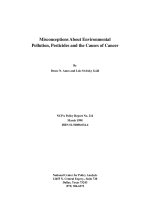
Figure 3 shows the maximum local R
2
from all seven
GWR analyses. The broad pattern introduced in Figure
1 of low values along the lower Mississippi River and in
Table 3 Multiple regression coefficients, standard errors (SE), and p-values.
Metropolitan Adjacent non- metropolitan Non-adjacent non- metropolitan
Coeff. (SE) P < Coeff. (SE) P < Coeff. (SE) P <
All-Cancer mortality 0.32 (.18) 0.08 0.38 (.28) 0.18 0.32 (.51) 0.53
Kidney disease mortality 0.14 (.08) 0.07 0.21 (.12) 0.08 0.55 (.18) 0.003
Total non-cancer mortality 1.21 (.82) 0.15 1.41 (1.20) 0.25 6.85 (2.17) 0.002
age-adjusted mortality rates and discharges by metropolitan status
Models control for college education rates, smoking rates, adult obesity rates, supply of primary care physicians, poverty rate, percent African American, percent
Native American, percent non-white Hispanic, percent Asian American, and percent other non-white race (percent white serving as the referent). Model F values
for all models significant at p < .0001
Table 4 Multiple regression results including covariates, for age-adjusted mortality rates and area-weighted and
toxicity weighted discharges

All-Cancer
mortality
1
Kidney disease
mortality
2
Total non- cancer
mortality
3
Coeff. (SE) P < Coeff. (SE) P < Coeff. (SE) P <
Log of non-carcinogen area weighted and toxicity
weighted discharges
NA – 0.25 (.06) <
0.0001
2.30 (.69) 0.0009
Log of carcinogen area weighted and toxicity
weighted discharges
0.35 (.16) 0.03 NA – NA –
Percent adults with college education -0.78 (.09) <
0.0001
-0.11 (.02) <
0.0001
-28 .5 <
0.0001
Adult smoking rate 1.24 (.12) <
0.0001
0.18 (.03) <
0.0001
3.25 (.35) <
0.0001

Adult obesity rate 0.43 (.18) 0.02 0.17 (.05) 0.002 2.88 (.52) <
0.0001
Per capita primary care doctors 1.83 (1.61) 0.26 -0.47 (.52) 0.37 7.03 (4.66) 0.14
Poverty rate 1.11 (.11) <
0.0001
0.20 (.03) <
0.0001
5.38 (.30) <
0.0001
Percent African American 0.20 (.04) <
0.0001
0.14 (.01) <
0.0001
1.50 (.12) <
0.0001
Percent Native American -0.22 (.08) 0.004 0.03 (.03) 0.23 0.45 (.22) 0.04
Percent Hispanic -0.91 (.09) <
0.0001
0.03 (.03) 0.36 -2.16 (.27) <
0.0001
Percent Asian American 0.65 (.34) 0.07 -0.19 (.09) 0.04 -0.07 (.99) 0.94
Percent other race 0.76 (.22) 0.0007 -0.17 (.07) 0.02 3.63 (.65) <
0.0001
Metropolitan county 9.98 (1.39) <
0.0001
0.02 (.40) 0.97 38.52 (4.03) <
0.0001
Adjacent, non- metropolitan county 1.90 (1.22) 0.12 -0.09 (.37) 0.82 9.00 (3.52) 0.02
1. Model F = 123.1 (df = 13, 3068), p < .0001; adjusted R-square = .34
2. Model F = 97.9 (df = 13, 2384), p < .0001; adjusted R-square = .34

3. Model F = 255.6 (df = 13, 3068), p < .0001; adjusted R-square = .52
Hendryx et al. International Journal of Health Geographics 2012, 11:9
/>Page 4 of 15
the Great Plains persists across all GWR results, along
with higher values along the Pacific coast and in parts
of the Midwest and Northeast. There is a wide range of
local R
2
values from less than 0.03 to greater than 0.65,
demonstrating that while the discharges and covariates
may correlate well with cancer mortality in some
regions of the country, they do not provide a strong cor-
relation nationwide. This also demonstrates that the
non-spatial analyses are masking substantial regional
variation in the correlations between these discharges
and health outcomes.
Figures 4, 5 and 6 shows the attributes of the measure
that led to the highest local R
2
value for each county. It
is broken down into each of the three propertie s of our
discharge measures: carcinogens versus no n-carcinogens
(Figure 4), on-site releases versus an area-weighted sum
of all upstream releases (Figure 5), and whethe r the
release amounts are weighted by toxicity values of the
chemicals discharged (Figure 6). Similar to Figure 3,
these maps illustrates the substantial variation from one
region of the country to another, as cancer mortality in
some parts of the country correlates better with the
onsite variables versus the area-weighted variables. Like-

wise, this correlation is stronger for non-carcinogens in
some regions and carcinogens in others. Thus, despite
the unexpected finding from the non-spatial analyses
that the non-carcinogens have a stronger correlation
with cancer mortality than carcinogens, this relationship
is not consistent for the entire country. There is no
strong pattern throughout the country.
Figure 4 reveals two br oad areas that do not conform
to the national trend of non-c arcinogens having a stron-
ger relat ionship with cancer mortality than carcinogens.
These regions, highlighted in red, are in the intermoun-
tain west and in parts of the Midwest extending to a
few places along the Atlantic Coast. Figure 5 does not
show a clear trend in on-site versus the area-weighted
sum of upstream releases, although three area s, the Mis-
sissippi River, Florida, and an area largely east of the
Appalachian Mountains extending from New York City
to South Carolina, show stronger on-site release effects.
For most of the United States, unsurprisingly, the toxi-
city-weighted measures have a stronger relati onship
with cancer mortality, as shown in Figure 6. However,
there are some regions in the Mid-Atlantic and southern
areas of the country, colored blue, where the toxicity
weights do not provide a stronger relationship.
Figure 7 shows the improvement in local R
2
over not
including any release variable. This illustrates how much
extra explanatory power the release variables give us
Figure 1 Local R-Square values for geographic-weighted regression results for cancer mortality and area weighted and toxicity-

weighted release.
Hendryx et al. International Journal of Health Geographics 2012, 11:9
/>Page 5 of 15
Figure 2 Local geographic-weighted regression coefficients for all-cancer mortality and area-weighted, toxicity-weighted carcinogenic
discharges.
Figure 3 Maximum local R
2
values for all-cancer mortality across all release variables.
Hendryx et al. International Journal of Health Geographics 2012, 11:9
/>Page 6 of 15
Figure 4 Regions where carcinogens versus non-carcinogens had the greatest local correlation with all-cancer mortality.
Figure 5 Regions where onsite releases in the county versus an area-weighted average of all upstream releases had the greatest local
correlation with all-cancer mortality.
Hendryx et al. International Journal of Health Geographics 2012, 11:9
/>Page 7 of 15
Figure 6 Regions where weighting the releases by toxicity versus not weighting the releases by toxicity had the greatest local
correlation with all-cancer mortality.
Figure 7 Improvement in local R-Square by including release variable.
Hendryx et al. International Journal of Health Geographics 2012, 11:9
/>Page 8 of 15
comp ared to the demographic data and other covariat es
listed in Table 1. As the map shows, about half the
country has very little improvement (less than 0.01
change in local R
2
), even from the best fitting release
variable. Cross-hatched areas are those where the best
fit was with the toxicity-weighted, area-weighted sum o f
non-carcinogenic releases, which is t he most significant
measure from the non-spatial results, and covers most

regions of the country that have the greatest improve-
ment from including pollution measures. Two large
areas of substantial improvement, northern New Eng-
land and the Northern Great Plains, both have the non-
carcinogen releases, weighted by toxicity, as the best fit.
This improvement is most dramatic in northern parts of
the Great Plains, downstream from the headwaters of
the Missouri and Yellowstone Rivers, which is a rural
area with very little onsite releases, but with greater
releases in the nearby upstream counties of Cascade and
Yellowstone in Montana, which contain the cities of
Great Falls and Billings respectively. Most counties in
New England and all in the Northern Plains have the
area-weighted measure as the best fit. Similarly, two less
substantial areas of improvement in the center of the
country and in the Pacific Northwest also relate to the
same measure. The exceptions to this pattern are an
are a in the northern Rocky Mountains where the onsite
toxicity-weighted release of carcinogens is highest, and
an area in the southwest, centered in Arizona, where
the area-weighted, non-toxicity-weighted releases of car-
cinogens are the strongest.
GWR analyses comparing the area-weighted non-carci-
nogen releases with total mortality were also conducted,
but are not shown in detail to conserve space. Further
information is available from the authors. The local R
2
values are higher than those for cancer mortality shown
in Figure 3, ranging from 0.09 to 0.79, although the spa-
tial pattern remains similar, with the highest values along

the Pacific and Atlantic coasts. This greater R
2
value is
due to the improved correlation between the covariates
and the mortality rate, as the local coefficient for the pol-
lution variable is non-significant for most of the country.
Only a small are a in the Great Plains and Midwest span-
ning from western South Dakota through Nebraska and
Iowa has a significantly positive coefficient and a signifi-
cantly negative coefficient is only located in the same
area of West Texas that has a significantly negative coef-
ficient in Figure 2.
Conclusions
The results of the non-spatial analyses suggest that per-
mitted discharges of chemical pollutants into surface
waters are related to higher adjusted population mortal-
ity rates. More specifically, total non-cancer mortality is
related to greater discharge quantities of chemicals
classified as non-carcinogenic without need for toxicity
weights or upstream discharges. For cancer mortality,
the toxicity wei ghts are necessary to detect associations
between carcinogenic discharges and death rates, and
for kidney disease mortality, both toxicity weights and
area-weighted upstream discharges are necessary to
detect discharge-mortality associations.
The cross-validation results suggest that chemicals not
currently recognized as carcinogens may nevertheless
play a role in contributing to cancer mortality risk. The
pot ential carcinogenic properties of many chemicals are
unknown and may be underestimated. Cross-validated

results for kidney disease were significant but at a
weaker level than for the non-cross-validation. There
was a significant correlation between higher carcinogen
releases and higher non-carcinogen releases (r = .69), so
the cross-validation analysis of kidney disease may still
be picking up non-carcinogen discharges. Some carcino-
gens such as cadmium or thallium are also recognized
as causes of kidney damage [11]. In contrast, the rela-
tively small subset of known or suspected carcinogens
was related to higher cancer mortality but not higher
non-cancer mortality.
Kidney and total non-cancer death rates are most
strongly related to discharges in rural areas not adjacent
to metropolitan areas as compared to other urban-rural
settings. It is possible that downstream effects from
urban to rural areas may be a contributing factor, or
downstream effects from one rural area to another.
The spatial analyses illustrate the wide variation of the
local R
2
values across the contiguous United States, as
well as the variation in which model has the most expla-
natory power. The effects of both the chemical discharges
and the covariates are not constant from one region of
the country to another. Spatial models generally support
the non-spatial analys is in that the releases of non-carci-
nogens are a better fit for the cancer mortality for most
of the country (2303 out of 3109 counties) than the
releases of carcinogens. For many of these counties, the
improvement over not including any release variable is

slight, indicating that the relative influence of chemical
surface water discharges is small compared to effects of
our covariates such as poverty or smoking rates. In many
of the regions for which the improvement in local R
2
was
greatest, that improvement comes from the area
weighted sum of all upstream releases of non-carcino-
gens, adjusted for toxicity. This suggests that for some,
but not all, parts of the country, upstream releases may
be an important factor.
A number of hypotheses may be suggested for future
research based on the findings. First, studies may under-
take whether chemicals currently not recognized as carci-
nogens may have carcinogenic properties. The number of
chemicals with established carcinogenic information,
Hendryx et al. International Journal of Health Geographics 2012, 11:9
/>Page 9 of 15
whether that information is confirmatory or not, is small
relative to the number of chemicals that are manufac-
tured or used [12] There are many chemicals used in
industrial processes or that are present in drinking water
for which we have no information on health risks. The
results of the current study can serve to encourage future
research on understanding the possible health impacts
for chemicals for which there is currently limited o r no
information. The choice o f which chemicals to investi-
gate may be guided by those which occur at highest
levels, those for which information on related chemical
properties suggests a possible health concern, or those

chemicals which are more prevalent in regions of the
country with the strongest relationship between the total
chemical discharges and cancer mortality.
Second, the effects of co-exposures or mixtures of
more than one chemical deserve further investigation.
Most exposure research has focused on the effects of a
single agent (lead, arsenic, benzo[a]pyrene, etc.), but
there is increasing recognition that exposures to multi-
pleagentssimultaneouslymorecloselymatcheswhat
people actually experience in daily life [13], and that co-
exposures may have additive or synergistic effects
beyond single exposures, although research on this
question is limited. The exposures in the current study
were not isolated as to single agents because of the large
number of possible agents to investigate and because
release levels of any particular agent expressed on a
national scale are usually sma ll and are often concen-
trated in a few regions of the country.
Based on previous research, investigations of co-expo-
sures may best be targeted initially to combinations of
single agents abou t which there are known effects, espe-
cially when those agen ts are known to have similar
health impacts such as manganese and lead co-exposure
impacting neurodevelopment [13], or studies that inves-
tigate mixtures of single agents that are known individu-
ally to increase cancer risk such as arsenic [14],
chromium(VI) [15], PAHs [16], tetrochloroethylene [17],
or others.
Third, regiona l variations seen in the curren t study are
intriguing but require future investigations to attempt to

understand. The northern Great Plains area highlighted in
Figure 5 is one example. This area is largely rural and
sparsely populated . It may be that rural areas, at least in
some circumstances, are less impacted by environmental
contaminants than urban area s, such that, when an
environmental pollutant source (such as PCS discharges)
is present i n a rural area, that source represents a
unique “ spike” in exposures relative to background,
whereas in urban areas with the same PCS pollutant
source, the additional contribution of this source to
health outcomes may be harder to detect against a
background of other pollutants from industry or
transportation.
Fourth, spatial variation in t he contributions of area-
weighted and on-site discharges suggests that area-
weighted or upstream discharges may be i mportant for
some areas, whereas local discharges are more impor-
tant for others (Figure 5). It is difficult to identify a pat-
tern that can account for this variation; on-sit e
discharges are relatively more important along the entire
Mississippi River, b ut other major river systems don’t
show this pattern. Some major population centers are in
areas where on-site discharges are more important, but
other population centers are in areas where area-
weighted scores had stronger effects. Regional variation
in the composition of chemicals discharged may play a
role in this spatial variati on, as some chemicals or com-
binations of interacting chemicals may be present in one
area but not in others. Regions to examine for these
effects include the Northern Rockies and Arizona,

where the measure of carcinogen releases instead of the
non-carcinogen releases added substantial explanatory
ability to the model , as well as areas in the Northern
Plains and New England, which showed the strongest
relationship between non-carcinogenic releases and can-
cer mortality. Similarly, there may be re gional variation
in how far downstream chemicals travel from the dis-
charge site. Both properties of the chemical, such as its
molecular weight, and properties of the stream, such as
how fast it is flowing , could affect the distance the che-
mical travels. Accounting for molecular weight of air-
borne pollutants can improve models of atmospheric
releases and public health outcomes [18], and a similar
strategy may be useful when examining water-borne
discharges.
Limits of the study include the ecological design, the
selection of a partial list of chemicals with ingestion
toxicity weights, the knowledge that the health impacts
of mixtures are poorly understood, and the imperfect
time relationships between discharges and mortality.
Kidney disease was selected as one diagnostic sub-group
for study but others, such as bladder cancer [19] could
also have been investigated. We do not account for
additional environmental variables that may be related
to cancer or non-cancer risks, including geographic var-
iatio n in levels of UV- B [20,21], nitrates from non-point
pollution agricultural sources [22], or traffic emissions.
The results of the study must be taken a s exploratory,
but do show possible connections between greater per-
mitted discharges of toxic chemicals into surface water

and human health consequences, with potentially
important geographic v ariations in the impacts of these
discharges and in the particular discharges and health
outcomes of greatest concern.
Hendryx et al. International Journal of Health Geographics 2012, 11:9
/>Page 10 of 15
Methods
Design
The study employs a county-level, ecological secondary
data analysis. Dependent variables are population age-
adjusted mortality rates (e.g., cancer mortality rates),
and are statistically associated with independent vari-
ables (e.g., releases of carcinogens into surface waters)
in the context of controlling for covariates (e.g., race/
ethnicity, poverty rates, physician supply). Variables are
described in further detail below.
The design also includes comparative findings for
rural and urban areas. Counties were classified using the
US Department of Agriculture’s urban-influence codes
(UICs) to identify metropolitan areas (codes 1 and 2),
non-metropolitan areas adjacent to metropolitan areas
(codes 3,4,5,6,7,9 and 10), and non-metropolitan areas
not adjacent to metropolitan areas (codes 8,11 and12).
Data sources and variables
The EPA’s Discharge Monitoring Report (DMR) data-
base, which includes data from the Permit Compliance
System (PCS) and the Integrated Compliance Informa-
tion System - National Pollutant Discharge Elimination
System (ICIS-NPDES), was used to measure the location,
type, and quantity of water pollution discharges [23]. The

DMR database provides infor mation on companies that
have been issued permits to discharge wastewater into
rivers or streams, including data on the amounts a nd
types of chemicals discharged. A n exported Oracle data-
base was provided to us by the EPA containing the DMR
data for the year 2007. The pollutant loading table in the
database included 322,113 records of aggregate discharge
measurements from 30,228 unique facilities. One thou-
sand one hundred nine (1,109) parameters are included
in the data, from basic water chemistry information (pH,
temperature, etc) to concentrations of various com-
pounds classified as “pollutants” by the EPA (n = 729).
Not all records contain values for all parameters; each
record contains values for one parameter, relevant to that
facilities’ permit. Of the pollutants, a total of 518 unique
Chemical Abstract Service (CAS) registry numbers were
identified in the data. Of those 518 CAS registry num-
bers, we initially limited the analysis to discharges of 73
chemicals selected based on their possible human health
impacts. We chose a subset of chemicals rather than
attempting to use all chemicals bec ause of the extensive
time demands required to find, clean, and aggregate che-
mical-specific discharge data across the 322,113 dis-
charge records in the DMR data. Selecting only those
records containing a chemical of interest left us with
55,183 records. We also limited the data points used in
the analysis by removing all records with a release value
across all chemicals of interest of zero (n = 20,948). Next,
we removed all records that fell outside of the contiguous
United States (n = 13,197), and all records whose lati-

tude/longitude coordinate fields contained values of “0”
or other anomalous values (n = 143). Finally, we removed
all records wherein a single facility listed the same dis-
charge value for all releases as this was clearly reported
in error (n = 56). Once these edits were completed, we
were left w ith a database of 19,824 permitted discharges
from 10,395 individual facilities which were used in
development of subsequent analyses.
To aggregate discharges from upstream sources into
downstream geographic areas, we utilized the Watershed
Boundary Dataset, a multi-level spatial dataset for water-
sheds created and maintained by the Natural Resource
ConservationService(NRCS)andpublishedaspartof
the National Hydrography Dataset (NHD) [24]. The data
were downloaded from the NHD server as a single file
for the United States. We extracted the Sixth level (12
digit) watershed and checked the relevant upstream and
downstream fields within the database to ensure that we
could connect the upstream to downstream flows.
Finally, we s ummed the discharges per chemical within
each watershed for use in later analysis and aggregation.
Toxicity weighted and un-weighted discharges
Chemicals vary in their toxicity, such that a given
amount of exposure may be harmless for one chemical
and deadly for another. Efforts have been undertake n to
estimate toxicity weights for specific chemicals [25]; cur-
rently there are weights a vailable for some but not all
chemicals included in the DMR database. From our
initial list we selected a ll 30 non-carcinogenic and all 8
carcinogenic chemicals with ingestion toxicity weights

as established by the EPA [26]. Carcinogens were
included if they were categorized as class 1, 2a or 2b by
the International Agency for Research on Cancer
(IARC)orasaKnownorProbablecarcinogenbythe
National Toxicology Program (NTP). For consistency,
analyses and reports presented in this paper for toxicity
weighted and non-weighted findings use the same sub-
set of 38 chemicals. The final list of chemicals with
weights is presented in Table 5. Although some of the
listed non-carcinogens have carcinogenic properties (e.
g., cadmium) we included only chemicals with estab-
lished toxicity weights for ingestion exposures, not inha-
lation exposures.
For toxicity weighted analyses, the values for each che-
mical were multiplied by the weight for that chemical.
Toxicity weighted and unweighted quantities for each
county were then summed across all carcinogens, and
again a cross all non-carcinogen chemicals. Amounts of
these summed chemical discharges were not normally
distributed across counties, so we calculated the natural
Hendryx et al. International Journal of Health Geographics 2012, 11:9
/>Page 11 of 15
log of discharge amounts for analysis. All dischar ges are
expressed as the log of kg per year.
Onsite and area-weighted upstream discharges
Onsite discharges were measured as the simple sum of
the log carcinogen and non-carcinogen chemical dis-
charges present in each county. These sums were com-
puted for both toxicity weighted and non-weighted
discharges. Discharges into waterways can flow down-

stream to impact communities where the re may be few
or even no on-site r eleases. To account for the impact
of upstream discharges, we develop a measure that
allows discharges to accumulate throughout a river sys-
tem. We also want to account for the likelihood that
releases upstream from a location will have a smaller
impact on that location than nearby releases. We per-
form this accounting by using a weighted sum of all
upstream releases, dividing e ach release by the area of
the watersheds between the release site and the impact
site. The following equation gives how this is calculated.
π
s
=

w≥s
ρ
w
area
w→s
Here, π
s
is the pollution score for the watershed, r
w
is
the summed releases for that watershed, w ≥ s denotes
all watersheds upstream of shed s, including shed s
itself, and area
w® S
denotes the area in acres of all

watersheds between sheds w and s, including both w
and s.Whenw = s, this reduces to the area of that
waters hed. We employ this reduction to account for the
likelihood that releases far upstream of a location will
have less influence on that location than nearby releases.
Population-weighted county-level discharges for both
onsite and areas-weighted upstream discharges
Because the demographic and mortality variables are
reported for each county, while the discharge variables
are calculated for each watershed, we transformed the
release variables from the smaller watersheds to county-
level summari es to conduct statistical an alysis at the
county level. A simple summation of the releases within
the counties is insufficient because of potential discre-
pancies within each county between where the residents
live and where the releases take place. As an extreme
example, imagine a county split between two watersheds;
the first watershed has all the releases but none of the
population, while the second watershed has all the popu-
lation but none of the releases. Even though there are
chemical discharges to streams within the county, none
of the population is exposed to those releases. Therefore,
we estimated the population living within each watershed
and county intersection. We used the LandScan Global
dataset [27 ] which estima tes populatio n at a grid with
cells approximately 1 km by 1 km in size. We then cre-
ated a population-weighted average exposure in each
county by applying the following formula:
e
c

=

s∩c
π
s
∗ pop
s,c

s∩c
pop
s,c
Here, s is a watershed, c is the county, pop
s, c
is the
estimated population in the watershed/county
Table 5 List of chemicals used in analyses
Chemical Name Toxicity Weight
Non-carcinogens 2,4-Dinitrophenol 500
1,1,1-Trichloroethane 0.5
Methoxychlor 200
1,1-Dichloroethylene 20
Hexachlorocyclopentadiene 170
Dinoseb 1000
2,4-D 200
o-Dichlorobenzene 11
1,2-Dibromo-3-chloropropane 5000
Styrene 5
Toluene 13
Chlorobenzene 50
Phenol 3.3

1,2,4-Trichlorobenzene 100
Xylene 5
Carbofuran 1200
Atrazine 56
Lead 18000
Manganese 7.1
Mercury 10000
Nickel 20
Thallium 14000
Antimony 2500
Barium 5
Beryllium 500
Cadmium 2000
Chromium 330
Copper 1500
Selenium 200
Chlorine 10
Carcinogens Lindane 110000
Benzene 55000
1,1,2-Trichloroethane 5700
Ethylbenzene 1100
p-Dichlorobenzene 2400
Di(2-ethylhexyl) phthalate 14000
Polychlorinated biphenyls 2000000
Arsenic 1500000
Hendryx et al. International Journal of Health Geographics 2012, 11:9
/>Page 12 of 15
intersection, π
s
is the pollution score for the watershed,

and e
c
is the total exposure score for the county. The
denominator of the fraction is simply the population of
the county, but is shown as the sum of the population
of all watershed/county intersections to illustrate the
weighted average nature of the calculation. We calcu-
lated values for both onsite and area-weighted expo-
sures. The onsite calculation replaces π
s
with the re lease
variable r
s
.
Outcome measures
HealthoutcomedataweredrawnfromthepublicCDC
mortality files for the years 2003-2007. We selected a
five-year aggregate period to acquire more stable esti-
mates than would be possible by selecting only one year,
and choose the most recent five-year period availa ble
from the CDC at the time of the study, recognizing that
this creates an imperfect match between the mortality
observation period and the chemical discharge period.
WeareforcedtoassumethatPCSdischargequantities
at the county level are stable over time, such that later
discharges provide a reasonable estimate of earlier
discharges.
From the CDC we found the annual age-adjusted
mortality rates per 100,000 for 1) all cancer (ICD-10
codes C00-C97 malignant neoplasms); 2) chronic or

unspecified non-cancer kidney disease (ICD-10 diagnos-
tic GR113 codes 99, 100 and 101; the uncommon c ode
98 reflecting ‘ acute and rapidly progressive’ disease was
excluded); and 3) all non-cancer mortality causes causes
combined, excluding accidents, suicide and homicide.
Kidney disease was selected as one category because of
previous research suggesting that kidney disease may be
particularly sensitive to exposure t o water pollutants,
especially heavy metals [28-31]. Rates were age-adjusted
using the standard 2000 US Census population.
Covariates
Other variables were measured from the 2007 Area
Resource File and CDC 2006 Behavioral Risk Factor Sur-
veil lance System (BRFSS) survey data. Covariates include
county-level measures of adult smoking rates, college
education rates, poverty rates, race/ethnicity percentages,
physician per capita supply, and adult obesity rates.
Analysis
Data analyses included calculation of descriptive statis-
tics and examination for multicollinearity, followed by
non-spatial and spatial analyses. For the non-spatial ana-
lyses, we examined associations between chemical dis-
charges and mortality through a series of linear multiple
regression models desig ned to build on o ne another to
test whether refinements to the specification of the dis-
charge variables improve d their capacity to account for
mortality rates. Spec ifically, we ran a series o f five sets
of analyses, and within e ach set we examined the three
primary outcomes of interest including cancer mortality
rates, total non-cancer mortality rates, and kidney dis-

ease mortality rates. In Sets 1 through 3 below, carcino-
gen discharges were used in models of cancer mortality
and non-carcinogen discharges were used in models of
non-cancer mortality. In Set 4, models were cross-vali-
dated by using carcinogen discharges in non- cancer
mortality models, and by using non-carcinogen dis-
charges in cancer mortality models. The five sets in
sequence were:
1. Onsite discharges not toxicity weighted
2. Onsite discharges with toxicity weights
3. Area weighted upstream discharges with toxicity
weights
4. Area weighted upstream discharges with toxicity
weights cross-validated.
5. Area weighted upstream discharges with toxicity
weights separately for metropolitan, non-metropolitan
adjacent, and non-metropolitan non-adjacent counties
Spatial analyses in cluded a series of seven geographi-
cally weighted regressions (GWR) [10,32]. This approach
recognizes that the relationships between the indepen-
dent and dependent variables in a standard regression
analysis may mask spatial variation in the relationships,
such that the relationship m ay be strong in one part of
the study area yet weak in another part. This could arise
in our study because we a re aggregating the releases of
many chemicals together, and spatial variation in the
composition of the chemical discharges could result in
spatial variation in the relationship between discharges
and public health outcomes. The GWR procedure cycles
through each county and conducts a multiple linear

regression for each county in the dataset, using o nly the
nearby counties. In this study, we used the 30 nearest
counties. This approach provides a local R
2
value and
local coefficients for each county based on its thirty
nearest n eighbors, rather than simply reporting a single
result for the entire dataset. Each of them compared
cancer mortality with the same demographic cova riates
as in the non-spatial regressions, and one o f the follow-
ing pollutant discharge variables.
A. Area weighted carcinogen releases, toxicity
weighted
B. Area weighted carcinogen releases, not toxicity
weighted
C. Area weighted non-carcinogen releases, toxicity
weighted
D. Onsite carcinogen releases, toxicity weighted
E. Onsite carcinogen releases not toxicity weighted
F. Onsite non-carcinogen releases, toxicity weighted
G. Onsite non-carcinogen releases not toxicity
weighted
Hendryx et al. International Journal of Health Geographics 2012, 11:9
/>Page 13 of 15
The eighth possible analysis, using the area weighted
non-carcinogen releases, not toxicity weighted, was not
completed because the GWR failed to evaluate because
of local multicollinearity errors, even w hen the number
of neighbors was increased to 300 counties. We did not
examine the geographic patterns of kidney mortality

because the suppression of some counties’ data due to
small numbers of cases precluded spatial analysis. We
decided to limit the spatial analysis to cancer mortality
to conserve space, but results for non-cancer mortality
are briefly described in text in the Results section.
Note
Support for this study was provided by the Office of
Rural Health Policy, Health Resources and Services
Administration, PHS Grant No. 1 U1CRH10664-01-00.
Author details
1
West Virginia Rural Health Research Center, West Virginia University,
Morgantown, USA.
2
Department of Community Medicine, West Virginia
University, Morgantown, USA.
3
Department of Geology and Geography, West
Virginia University, Morgantown, USA.
4
Department of Community Medicine,
West Virginia University, PO Box 9190, Morgantown, WV 26505, USA.
Authors’ contributions
MH conceived the study and contributed to the design, analysis,
interpretation of results, and writing the manuscript. JC led the spatial
analysis and contributed to interpretation of results and writing. EF
contributed to the spatial analysis, interpretation of results and writing. JL
contributed to the statistical analysis, interpretation of results and writing.
MA contributed to database creation, study design, and writing. All authors
read and approved the final manuscript.

Competing interests
The authors declare that they have no competing interests.
Received: 23 February 2012 Accepted: 2 April 2012
Published: 2 April 2012
References
1. Hendryx M, Fedorko E, Halverson J: Pollution sources and mortality rates
across rural-urban areas in the United States. J Rural Health 2010,
26:383-391.
2. Strange C, Fedorko E, Hendryx M: Downstream cancer mortality: using
geospatial techniques to examine point source pollution impacts within
the Ohio River watershed. Presented at the American Association of Public
Health Annual Meeting, Philadelphia 2009.
3. Tornqvist R, Jerker J, Karimov B: Health risks from large-scale water
pollution: trends in Central Asia. Environ Int 2011, 37:435-442.
4. Cantor KP: Drinking water and cancer. Cancer Causes Control 1997,
8:292-308.
5. Rahman MM, Ng JC, Naidu R: Chronic exposure of arsenic via drinking
water and its adverse health impacts on humans. Environ Geochem
Health 2009, 31(Suppl 1):189-200.
6. Griffith J, Duncan RC, Riggan WB, Pellom AC: Cancer mortality in US
counties with hazardous waste sites and ground water pollution. Arch
Environ Health 1989, 44(2):69-74.
7. Vrijheid M: Health effects of residence near hazardous waste landfill
sites: a review of epidemiologic literature. Environ Health Perspect 2000,
108(Suppl 1):101-112.
8. VanDerslice J: Drinking water infrastructure and environmental
disparities: evidence and methodological considerations. Am J Public
Health 2011, 101(Suppl 1):S109-S114.
9. Winter WC, Harvey JW, Franke OL, Alley WM: Ground water and surface
water: a single resource. US Geological Survey Circular 1139 1998 [http://

pubs.usgs.gov/circ/circ1139/], [Accessed 11-14-11.].
10. Brunsdon C, Fotheringham S, Charlton M: Geographically weighted
regression–modeling spatial non-stationarity. The Statistician 1998,
47:431-443.
11. EPA: Drinking Water Contaminants. Environmental Protection Agency.
[ [Accessed 09-30-
11].
12. Environmental Working Group: National Drinking Water Database -
Executive Summary.[ />[Accessed 02-09-12].
13. Henn BC, Schnaas L, Ettinger AS, Schwartz J, Lamadrid-Figueroa H,
Hernandez-Avila M, et al: Associations of early childhood manganese and
lead coexposure with neurodevelopment. Environ Health Perspect 2012,
120:126-131.
14. Meliker JR, Slotnick MJ, AvRuskin GA, Schottenfeld D, Jacquez GM,
Wilson ML, Goovaerts P, Franzblau A, Nriagu JO: Lifetime exposure to
arsenic in drinking water and bladder cancer: a population-based case-
control study in Michigan, USA. Cancer Causes Control 2010, 21:745-757.
15. Zhitkovich A: Chromium in drinking water: sources, metabolism, and
cancer risks. Chem
Res Toxicol 2011, 24:1617-1629.
16. Grant WB: Air pollution in relation to U.S. cancer mortality rates: an
ecological study; likely role of carbonaceous aerosols and polycyclic
aromatic hydrocarbons. Anticancer Res 2009, 29:3537-3545.
17. Gallagher LG, Vieira VM, Ozonoff D, Webster TF, Aschengrau A: Risk of
breast cancer following exposure to tetrachloroethylene-contaminated
drinking water in Cape Cod. Massachusetts: reanalysis of a case-control
study using a modified exposure assessment. Environ Health 2011, 10:47.
18. Conley JF, Stewart RN: Using fine resolution population data and spatial
interaction modeling to estimate risk from airborne toxic releases.
Eleventh International Conference on GeoComputation, London, UK 2011.

19. Guo HR: Age adjustment in ecological studies: using a study on arsenic
ingestion and bladder cancer as an example. BMC Public Health 2011,
11:820, doi: 10.1186/1471-2458-11-820.
20. Grant WB: An estimate of premature cancer mortality in the U.S. due to
inadequate doses of solar ultraviolet-B radiation. Cancer 2002,
94:1867-1875.
21. Grant WB, Garland CF: The association of solar ultraviolet B (UVB) with
reducing risk of cancer: multifactorial ecologic analysis of geographic
variation in age-adjusted cancer mortality rates. Anticancer Res 2006,
26:2687-2699.
22. Ward MH: Too much of a good thing? Nitrate from nitrogen fertilizers
and cancer. Rev Environ Health 2009, 24:357-363.
23. EPA: Discharge Monitoring Report Pollutant Loading Tool. Environmental
Protection Agency [ [Accessed 10-18-11.].
24. NRCS: Watershed Boundary Dataset. Natural Resources Conservation Service,
US Department of Agriculture [ />main/national/water/watersheds/dataset], [Accessed 10-18-11.].
25. Lim SR, Lam CW, Schoenung JM: Quantity-based and toxicity-based
evaluation of the U.S. Toxics Release Inventory. J Hazard Mater 2010,
178:49-56.
26. Risk Screening Environmental Indicators (RSEI): Environmental Protection
Agency. Technical Appendix A: Listing of all toxicity weights for TRI
chemicals and chemical categories.[ />technical_appendixa_toxicity.pdf], [Accessed 11-14-11].
27. Dobson JE, Bright EA, Coleman PR, Durfee RC, Worley BA: A global
population database for estimating populations at risk. Photogramm Eng
Rem Sens 2000, 66:849-857.
28. Nwankwo EA, Ummate I: Environmental lead intoxication and chronic
kidney disease: a review. Internet J Nephrol 2006, 3(1)[ub.
com:80/journal/the-internet-journal-of-nephrology/volume-3-number- 1/
environmental-lead-intoxication-and-chronic-kidney-disease-a-review.html],
[Accessed 03-28-12.].

29. Hodgson S, Nieuwenhuijsen MJ, Elliott P, Jarup L: Kidney disease mortality
and environmental exposure to mercury. Am J Epidemiol 2006, 165:72-77.
30. Cadmium. CAS # 7440-43-9:
Agency for Toxic Substance and Disease
Registry. Division
of Toxicology and Environmental Medicine ToxFAQs 2008.
31. Meliker JR, Wahl RL, Cameron LL, Nriagu JO: Arsenic in drinking water and
cerebrovascular disease, diabetes mellitus, and kidney disease in
Michigan: a standardized mortality ratio analysis. Environ Health 2007,
Hendryx et al. International Journal of Health Geographics 2012, 11:9
/>Page 14 of 15
6(4)[ doi:10.1186/1476-069X-6-4.
[Accessed 03-28-12.].
32. Fotheringham AS, Brunsdon C, Charlton M: Geographically Weighted
Regression: The Analysis of Spatially Varying Relationships Chichester, England:
John Wiley & Sons Ltd.; 2002.
doi:10.1186/1476-072X-11-9
Cite this article as: Hendryx et al.: Permitted water pollution discharges
and population cancer and non-cancer mortality: toxicity weights and
upstream discharge effects in US rural-urban areas. International Journal
of Health Geographics 2012 11:9.
Submit your next manuscript to BioMed Central
and take full advantage of:
• Convenient online submission
• Thorough peer review
• No space constraints or color figure charges
• Immediate publication on acceptance
• Inclusion in PubMed, CAS, Scopus and Google Scholar
• Research which is freely available for redistribution
Submit your manuscript at

www.biomedcentral.com/submit
Hendryx et al. International Journal of Health Geographics 2012, 11:9
/>Page 15 of 15