Updating a Cracked Database potx
Bạn đang xem bản rút gọn của tài liệu. Xem và tải ngay bản đầy đủ của tài liệu tại đây (1.65 MB, 12 trang )
Updating a Cracked Database
Stratos Idreos
CWI Amsterdam
The Netherlands
Martin L. Kersten
CWI Amsterdam
The Netherlands
Stefan Manegold
CWI Amsterdam
The Netherlands
ABSTRACT
A cracked database is a datastore continuously reorganized
based on operations being executed. For each query, the
data of interest is physically reclustered to speed-up future
access to the same, overlapping or even disjoint data. This
way, a cracking DBMS self-organizes and adapts itself to the
workload.
So far, cracking has been considered for static databases
only. In this paper, we introduce several novel algorithms
for high-volume insertions, deletions and updates against
a cracked database. We show that the nice performance
prop e rties of a cracked database can be maintained in a
dynamic environment where updates interleave with queries.
Our algorithms comply with the cracking philosophy, i.e., a
table is informed on pending insertions and deletions, but
only when the relevant data is needed for query processing
just enough pending update actions are applied.
We discuss details of our implementation in the context of
an open-source DBMS and we show through a detailed ex-
perimental evaluation that our algorithms always manage to
keep the cost of querying a cracked datastore with pending
updates lower than the non-cracked case.
Categories and Subject Descriptors: H.2 [DATABASE
MANAGEMENT]: Physical Design - Systems
General Terms: Algorithms, Performance, Design
Keywords: Database Cracking, Self-organization, Updates
1. INTRODUCTION
During the last years, more and more database researchers
acknowledge the need for a next generation of database
systems with a collection of self-* properties [4]. Future
database systems should b e able to self-organize in the way
they manage resources, store data and answer queries. So
far, attempts to create adaptive database systems are based
either on continuous monitoring and manual tuning by a
database administrator or on offline semi-automatic work-
load analysis tools [1, 12].
Permission to make digital or hard copies of all or part of this work for
personal or classroom use is granted without fee provided that copies are
not made or distributed for profit or commercial advantage and that copies
bear this notice and the full citation on the first page. To copy otherwise, to
republish, to post on servers or to redistribute to lists, requires prior specific
permission and/or a fee.
SIGMOD’07, June 11–14, 2007, Beijing, China.
Copyright 2007 ACM 978-1-59593-686-8/07/0006 $5.00.
Recently, database cracking has been proposed in the con-
text of column-oriented databases as a promising di rection
to create a self-organizing database [6]. In [5], the authors
prop os e, implement and evaluate a query processing archi-
tecture based on cracking to prove the feasibility of the vi-
sion. The main idea is that the way data is physically stored
is continuously changing as queries arrive. All qualifying
data (for a given query) is clustered in a contiguous space.
Cracking is applied at the attribute level, thus a query re-
sults in physically reorganizing the column (or columns) ref-
erenced, and not the complete table.
The following simplified example shows the potential ben-
efits of cracking in a column-store setting. Assume a query
that requests A < 10 from a table. A cracking DBMS clus-
ters all tuples of A with A < 10 at the beginning of the
column, pushing all tuples with A ≥ 10 to the end. A future
query requesting A > v
1
, where v
1
≥ 10, has to search only
the last part of the column where values A ≥ 10 exist. Sim-
ilarly, a future query that requests A < v
2
, where v
2
< 10,
has to search only the first part of the column. To make this
work we need to maintain a navigational map derived from
all queries processed so far. The terminology “cracking” re-
flects the fact that the database is partitioned/cracked into
smaller and manageable pieces.
In this way, data access becomes significantly faster with
each query being processed. Only the first query suffers from
lack of navigational advice. It runs slightly slower compared
to the non-cracked case, because it has to scan and physi-
cally reorganize the whole column. All subsequent queries
can use the navigational map to limit visiting pieces for fur-
ther cracking. Thus, every executed query makes future
queries run faster.
In addition to query speedup, cracking gives a DBMS the
ability to self-organize and adapt more easily. When a part
of the data becomes a hotspot (i.e., queries focus on a small
database fragment) physical storage and automatically col-
lected navigational advice improve access times. Similarly,
for dead areas in the database it can drop the navigational
advice. No external (human) administration or a priori
workload knowledge is required and no initial investment
is needed to create index structures. Such properties are
very desirable for databases with huge data sets (e.g., scien-
tific databases), where index selection and maintenance is a
daunting task.
Cracked databases naturally seem to be a promising direc-
tion to realize databases with self-* properties. Until now,
database cracking has been studied for the static scenario,
i.e., without updates [6, 5]. A new database architecture
should also handle high-volume updates to be considered as
a viable alternative.
The contributions of this paper are the following. We
present a series of algorithms to supp ort insertions, dele-
tions and updates in a cracking DBMS. We show that our
algorithms manage to maintain the advantage of cracking
in terms of fast data access. In addition, our algorithms do
not hamper the ability of a cracking DBMS to s elf-organize,
i.e., the system can adapt to query workload with the same
efficiency as before and still with no external administra-
tion. The proposed algorithms fol low the “cracking philos-
ophy”, i.e., unless the system is idle, we always try to avoid
doing work until it is unavoidable. In this way, incoming
updates are simply marked as pending actions. We update
the “cracking” data structures once queries have to inspect
the updated data. The proposed algorithms range from the
complete case, where we appl y all pending actions i n one
step, to solutions that update only what is really necessary
for the current query; the rest is left for the future when
users will become interested in this part of the data.
We implemented and evaluated our algorithms using Mon-
etDB [13], an open source column-oriented database system.
A detailed experimental evaluation demonstrates that up-
dates can indeed be handled efficiently in a cracking DBMS.
Our study is based on two performance metrics to character-
ize system behavior. We observe the total time needed for
a query and up date sequence, and our second metric is the
per query response time. The query response time is crucial
for predictability, i.e., ideally we would like similar queries
to have a similar response time. We show that it is possible
to sacrifice little from the performance in terms of total cost
and to keep the response time in a predictable range for all
queries.
Finally, we discuss various aspects of our implementation
to show the algorithmic complexity of supporting updates.
A direct comparison with an AVL-tree based scheme high-
lights the savings obtained with the cracking philosophy.
The rest of the paper is organized as follows. In Sec-
tion 2, we shortly recap the experimentation system, Mon-
etDB, and the basics of the cracking architecture. In Sec-
tion 3, we discuss how we fitted the update process into the
cracking architecture by extending the select operator. Sec-
tion 4 presents a series of algorithms to support insertions
in a cracked database. Then, in Section 5, we present algo-
rithms to handle deletions, while in Section 6 we show how
updates are processed. In Section 7, we present a detailed
experimental evaluation. Section 8 discusses related work
and finally Section 9 discusses future work directions and
concludes the paper.
2. BACKGROUND
In this section, we provide the necessary background knowl-
edge on the system architecture being used for this study
and the cracking data structure.
2.1 Experimentation platform
Our experimentation platform is the open-source, rela-
tional database system MonetDB, which represents a mem-
ber of the class of column-oriented data stores [10, 13]. In
this system every relational table is represented as a collec-
tion of, so called Binary Association Tables (BATs). For a
relation R of k attributes, there exist k BATs. Each BAT
holds key-value pairs. The key identifies values that belong
to the same tuple through all k BATs of R, while the value
part is the actual attribute stored. Typically, key values are
a dense ascending sequence, which enables MonetDB to (a)
have fast positional lookups in a BAT given a key and (b)
avoid materializing the key part of a BAT in many situations
completely. To enable fast cache-conscious scans, BATs are
stored as dense tuple sequences. A detailed description of
the MonetDB architecture can be found in [3].
2.2 Cracking architecture
The idea of cracking was originally introduced in [6]. In
this paper, we adopt the cracking technique for column-
oriented databases proposed in [5] as the basis for our im-
plementation. In a nutshell, it works as follows. The first
time an attribute A is required by a query, a cracking DBMS
creates a copy of column A, called the cracker column of A.
From there on, cracking, i.e., physical reorganization for the
given attribute, happens on the cracker column. The orig-
inal column is left as is, i.e., tuples are ordered according
to their insertion sequence. This order is exploited for fast
reconstruction of records, which is crucial so as to maintain
fast q uery processing speeds in a column-oriented database.
For each cracker column, there exists a cracker index that
holds an ordered list of position-value (p, v) pairs for each
cracked piece. After position p all values in the cracker col-
umn of A are greater than v. The cracker index is imple-
mented as an in memory AVL-tree and represents a sparse
clustered index.
Partial physical reorganization of the cracker column hap-
pens every time a query touches the relevant attribute. In
this way, cracking is integrated in the critical path of query
execution. The index determines the pieces to be cracked
(if any) when a query arrives and is updated after every
physical reorganization on the cracker column.
Cracking can be implemented in the relational algebra en-
gine using a new pipe-line operator or, in MonetDB’s case, a
modification to its implementation of the relational algebra
primitives. In this paper, we focus on the select operator,
which in [5] has been ex tended with a few steps in the fol-
lowing order: search the cracker index to find the pieces of
interest in a cracker column C, physically reorganize some
pieces to cluster the result in a contiguous area w of C, up-
date the cracker index, and return a BAT (view) of w as
result. Although, more logical steps are involved than with
a simple scan-select operator, cracking is faster as it has to
access only a restricted part of the column (at most two
pieces per query).
3. UPDATE-AWARE SELECT OPERATOR
Having briefly introduced our experimentation platform
and the cracking approach, we continue with our contribu-
tions, i.e., updates in a cracking DBMS. Updating the ori gi-
nal columns is not affected by cracking, as a cracker column
is a copy of the respe ctive original column. Hence, we as-
sume that updates have already been applied to the original
column before they have to be applied to the cracker column
and cracker index. In the remainder of this paper we focus
on updating the cracking data structures only.
There are two main issues to consider: (a) when and (b)
how the cracking data structures are updated. Here, we
discuss the first issue, postponing the latter to Section 4.
One of the key points of the cracking architecture is that
physical reorganization happens with every query. However,
each query causes only data relevant for its result to be phys-
ically reorganized. Using this structure, a cracking DBMS
has the ability to s elf-organize and adapt to query workload.
Our goal is to maintain these properties also in the pres-
ence of updates. Thus, the architecture proposed for up-
dates is in line with the cracking philosophy, i.e., always do
just enough. A part of a cracker column is never updated
before a user is interested in its actual value. Updating the
database becomes part of query execution in the same way
as physical reorganization entered the critical path of query
pro ces si ng.
Let us proceed with the details of our architecture. The
cracker column and index are not immediately updated as
requests arrive. Instead, updates are kept in two separate
columns for each attribute: the pending insertions column
and the pending deletions colum n. When an insert request
arrives, the new tuples are simply appended to the rele-
vant pending insertions column. Simil arly, the tuples to be
deleted are appended in the pending deletions column of the
referred attribute. Finally, an update query is simply trans-
lated into a deletion and an insertion. Thus, all update
op e rations can be executed very fast, since they result in
simple append operations to the pending-update columns.
When a query requests data from an attribute, the rele-
vant cracking data structures are updated if necessary. For
example, if there are pending insertions that qualify to be
part of the result, then one of the cracker update algorithms
(cf., Sections 4 & 5) is triggered to make sure that a complete
and correct result can be returned. To achieve this goal, we
integrated our algorithms in a cracker-aware version of the
select operator in MonetDB. The exact steps of this operator
are as follows: (1) search the pending insertions column to
find qualifying tuples that should be included in the result,
(2) search the pending deletions column to find qualifying
tuples that should be removed from the result, (3) if at least
one of the previous results is not empty, then run an update
algorithm, (4) search the cracker index to find which pieces
contain the query boundaries, (5) physically reorganize these
pieces (at most 2) and (6) return the result.
Steps 1, 2 and 3 are our extension to support updates,
while Steps 4, 5 and 6 are the original cracker select op-
erator steps as proposed in [5]. When the select operator
pro cee ds with Step 4, any pending insertions that should be
part of the result have been placed in the cracker column
and removed from the pending insertions column. Likewise,
any pending deletions that should not appear in the result
have been removed form the cracker column and the pending
deletions column. Thus, the pending columns continuously
shrink when queries consume updates. They grow again
with incoming new updates.
Up dates are received by the cracker data structures only
upon commit, outside the transaction boundaries. By then,
they have also been applied to the attribute columns, which
means that the pending cracker column updates (and cracker
index) can always be thrown away without loss of informa-
tion. Thus, in the same way that cracking can be seen as
dynamically building an index based on query workload, the
update-aware cracking architecture proposed can be seen as
dynamically updating the index based on query workload.
4. INSERTIONS
Let us proceed our discussion on how to update the crack-
ing data structures. For ease of presentation, we first present
algorithms to handle insertions. Deletions are discussed in
Section 5 and updates in Section 6. We discuss the general
issues first, e.g., what is our goal, which data structures do
we have to update, how etc. Then, a series of cracker update
algorithms are presented in detail .
4.1 General discussion
As discussed in Section 2, there are two basic structures
to consider for updates in a cracking DBMS, (a) the cracker
column and (b) the cracker index. A cracker index I main-
tains information about the various pieces of a cracker col-
umn C . Thus, if we insert a new tuple in any position of C,
we have to update the information of I appropriately. We
discuss two approaches in detail: one that makes no effort
to maintain the index, and a second that always tries to
have a valid (cracker-column,cracker-index) pair for a given
attribute.
Pending insertions column. To comply with the “crack-
ing philosophy”, all algorithms start to update the cracker
data structures once a query requests values from the pend-
ing insertions column. Hence, looking up the requested
value ranges in the pending insertions column must be effi-
cient. To ensure this, we sort the pending insertions column
once the first query arrives after a sequence of updates, and
then exploit binary search. Our merging algorithms keep
the pending insertions column sorted. This approach is ef-
ficient as the pending insertions column is usually rather
small compared to the complete cracker column, and thus,
can be kept and managed in memory. We leave further anal-
ysis of alternative techniques — e.g., applying cracking with
“instant updates” on the p ending insertions column — for
future research.
Discarding th e cracker index. Let us b egin with a
naive algorithm, i.e., the forget algori thm (FO). The idea
is as follows. When a query requests a value range such
that one or more tuples are contained in the pending inser-
tions column, then FO will (a) compl etely delete (forget)
the cracker index and (b) simply append all pending inser-
tions to the cracker column. This is a simple and very fast
op e ration. Since the cracker index is now gone, the cracker
column is again valid. From there on, the cracker index is
rebuilt from scratch as future queries arrive. The query that
triggered FO performs the first cracking operation and goes
through all the tuples of the cracker column. The effect is
that a number of queries suffer a higher cost, compared to
the performance before FO ran, since they will physically
reorganize large parts of the cracker column again.
Cracker index maintenance Ideally, we would like to
handle the appropriate insertions for a given query with-
out loosing any information from the cracker index. Then,
we could continue answering queries fast without having a
number of queries after an update with a higher cost. This
is desirable not only because of speed, but also to be able
to guarantee a certain level of predictability in terms of re-
sponse time, i.e., we would like the system to have similar
performance for similar queries. This calls for a merge-like
strategy that “inserts” any new tuple into the correct posi-
tion of a cracker column and correctly updates (if necessary)
its cracker index accordingly.
A simple example of such a “lossless” insertion is shown in
Figure 1. The left-hand part of the figure depicts a cracker
column, the relevant information kept in its cracker index,
and the pending insertions column. For simplicity, a single
3
2
9
8
7
15
35
19
37
56
43
60
58
89
59
97
95
91
99
Cracker column
Piece 1
Piece 2
Piece 3
Piece 4
Piece 5
Pos
1
2
3
4
5
6
7
8
9
10
11
12
13
14
15
16
17
18
19
20
Information in the
cracker index
start position: 1
values: <=12
start position: 6
values: > 12
start position: 10
values: > 41
start position: 12
values: > 56
start position: 16
values: > 90
Pending
Insertions
17
(a) Before the insertion
3
2
9
8
7
15
35
19
37
17
56
43
60
58
89
59
97
95
91
99
Cracker column
Piece 1
Piece 2
Piece 3
Piece 4
Piece 5
Pos
1
2
3
4
5
6
7
8
9
10
11
12
13
14
15
16
17
18
19
20
Information in the
cracker index
start position: 1
values: <=12
start position: 6
values: > 12
start position: 11
values: > 41
start position: 13
values: > 56
start position: 17
values: > 90
(b) After inserting value 17
Figure 1: An example of a lossless insertion for a
query that requests 5 < A < 50
pending insert with value 17 is considered. Assume now a
query that requests 5 < A < 50, thus the pending insert
qualifies and should be part of the result. In the right-hand
part of the figure, we s ee the effect of merging value 17
into the cracker column. The tuple has been placed in the
second cracker piece, since, according to the cracker i ndex,
this piece holds all tuples with value v, where 12 < v ≤ 41.
Notice, that the cracker index has changed, too. Information
ab out Pieces 3, 4 and 5 has been updated, increasing the
respective starting positions by 1.
Trying to device an algorithm to achieve this behavior,
triggers the problem of moving tuples in different positions
of a cracker column. Obviously, large shifts are too costly
and should be avoided. In our example, we moved down
by one position all tuples after the insertion point. This is
not a viable solution in large databases. In the rest of this
section, we discuss how this merging step can be made very
fast by exploiting the cracker index.
4.2 Shuffling a cracker column
We make the following observation. Inside each piece of
a cracker column, tuples have no specific order. This means
that a cracker piece p can be shifted z positions down in a
cracker column as follows. Assume that p holds k tuples.
If k ≤ z, we obviously cannot do better than moving p
completely, i.e., all k tuples. However, in case k > z, we can
take z tuples from the beginning of p and move them to the
end of p. This way, we avoid moving all k tuples of p, but
move only z tuples. We will call this technique shuffling.
In the example of Figure 1 (without shuffling), 10 tuples
are moved down by one position. With shuffling we need to
move only 3 tuples. Let us go through this example again,
this time using shuffling to see why. We start from the last
piece, Piece 5. The new tuple with value 17 does not belong
there. To make room for the new tuple further up in the
cracker column, the first tuple of Piece 5, t
1
, is moved to
the end of the column, freeing its original position p
1
to be
used by another tuple. We continue with Piece 4. The new
tuple does not belong here, either, so the first tuple of Piece
4 (position p
2
), is moved to position p
1
. Position p
2
has
become free, and we proceed with Piece 3. Again the new
tuple does not belong here, and we move the first tuple of
Piece 3 (position p
3
) to position p
2
. Moving to Piece 2, we
see that value 17 belongs there, s o the new tuple is placed
Algorithm 1 Merge(C,I,posL,posH)
Merge t he cracker column C with the pending insertions column
I. Use the tuples of I between positions posL and posH in I.
1: remaining = posH - posL +1
2: ins = poi nt at position posH of I
3: next = point at the last position of C
4: prevP os = the position of the last value in C
5: while remaining > 0 do
6: node = getPieceThatT hisBelongs(value(next))
7: if node == first piece then
8: break
9: end if
10: write = point one position after next
11: cur = point remaining − 1 positions after write in C
12: while remaining > 0 and
(v alue(ins) > node.value or
(v alue(ins) == node.value and node.incl == true)) do
13: move ins at the position of cur
14: cur = point at previous position
15: ins = point at previous position
16: remaining − −
17: end while
18: if remaining == 0 then
19: break
20: end if
21: next = point at p ositi on node.position in C
22: tuples = prevP os - node.position
23: cur = point one position after next
24: if tuples > remaining then
25: w = point at the position of write
26: copy = remaining
27: else
28: w = point remaining − tuples positions after write
29: copy = tuples
30: end if
31: for i = 0; i < copy; i + + do
32: move cur at the position of w
33: cur = point at previous position
34: w = point at previous position
35: end for
36: prevP os = node.position
37: node.position+ = remaining
38: end while
39: if node == first piece and remaining > 0 then
40: w = point at position posL
41: write = point one position after next
42: for i = 0; i < remaining; i + + do
43: move cur at the position of w
44: cur = point at next position
45: w = point at next position
46: end for
47: end if
in position p
3
at the end of Piece 2. Finally, the information
in the cracker index is updated so that Pieces 3, 4 and 5
have their starting positions increased by one. Thus, only 3
moves were made this time. This advantage becomes even
bigger when inserting multiple tuples in one go.
Algorithm 1 contains the details to merge a sorted por-
tion of a pending insertions column into a cracker column.
In general, the procedure starts from the last piece of the
cracker column and moves its way up. In each piece p, the
first step is to place at the end of p any pending insertions
that belong there. Then, remaining tuples are moved from
the beginning of p to the end of p. The variable remaining
is initially equal to the number of insertions to be merged
and is decreased for each insertion put in place. The process
continues as long as there are pending insertion to merge.
If the first piece is reached and there are still pending inser-
tions to merge, then all remaining tuples are placed at the
end of the first piece. This procedure is the basis for all our
merge-like insertion algorithms.
4.3 Merge-like algorithms
Based on the above shuffling technique, we design three
merge-like algorithms that differ in the amount of pending
insertions they merge per query, and in the way they make
ro om for the pending insertions in the cracker column.
MCI. Our first algorithm is called merge completely in-
sertions. Once a query requests any value from the pending
insertions column, it is merged completely, i.e., all pending
insertions are placed in the cracker column. The disadvan-
tage is that MCI “punishes” a single query with the task to
merge all currently pending insertions, i.e., the first query
that needs to touch the pending insertions after the new tu-
ples arrived. To run MCI, Algorithm 1 is called for the full
size of the pending insertions column.
MGI. Our second algorithm, merge gradually insertions,
go es one step further. In MGI, if a query needs to touch
k tuples from the pending insertions column, it will merge
only these k tuples into the cracker column, and not all
pending insertions. The remaining pending insertions wait
for future queries to consume them. Thus, MGI does not
burden a single query to merge all pending insertions. For
MGI, Algorithm 1 runs for only a portion of the pending
insertions column that qualifies as query result.
MRI. Our third algorithm is called merge ripple inser-
tions. The basic idea behind MRI is triggered by the follow-
ing observation about MCI and MGI. In general, there is a
number of pieces in the cracker column that we shift down
by shuffling until we start merging. These are all the pieces
from the end of the column until the piece p
h
where the tuple
with the highest qualify ing value belongs to. These pieces
are irrelevant for the current query since they are outside
the desired value range. All we want, regarding the current
query, is to make enough room for the insertions we must
merge. This is exactly why we shift these pieces down.
To merge k values MRI starts directly at the position that
is after the last tuple of piece p
h
. From there, k tuples are
moved into a temporary space temp. Then, the procedure
of Algorithm 1 runs for the qualifying portion of the pend-
ing insertions as in MGI. The only difference is that now the
pro cedure starts merging from piece p
h
and not from the last
piece of the cracker column. Finally, the tuples in temp are
merged into the pending insertions column. Merging these
tuples back in the cracker column is left for future queries.
Note, that for a query q, all tuples in temp have values
greater than the pending insertions that had to be merged
in the cracker column because of q (since these tuples are
taken from after piece p
h
). This way, the pending insertions
column is continuously filled with tuples with increasing val-
ues up to a point where we can simply append these tuples at
the cracker column without affecting the cracker index (i.e.,
tuples that belong to the l ast piece of the cracker column).
Let us go through the example of Figure 1 again, using
MRI this time. Piece 3 contains the tuple with the highest
qualifying value. We have to merge tuple t with value 17.
The tuple with value 60 is moved from position 12 in the
cracker column to a temporary space. Then the procedure
of Algorithm 1 starts from Piece 3. t does not belong in
Piece 3 so the tuple with value 56 is moved from position
10 (the first position of Piece 3) to position 12. Then, we
continue with Piece 2. t belongs there so it is simply placed
in position 10. The cracker index is also updated so that
Pieces 3 and 4 have their starting positions increased by
one. Finally, the tuple with value 60 is moved from the
temporary space to the pending insertions. At this point
MRI finishes without having shifted Pieces 4 and 5 as MCI
and MGI would have done.
In Section 7, a detailed analysis is provided that clearly
shows the advantage of MRI by avoiding the unnecessary
shifting of non-interesting pieces. Of course, the perfor-
mance of all algorithms highly depends on the scenario, e.g.,
how often updates arrive, how many of them and how often
queries ask for the values used in the new tuples. We exam-
ine various scenarios and show that all merge-like algorithms
always outperform the non-cracking and AVL-case.
5. DELETIONS
Deletion operations form the counter-part of i nsertions
and they are handled in the same way, i.e., when a new
delete query arrives to delete a tuple d from an attribute
A, it is simply appended to the pending deletions column of
A. Only once a query requests tuples of A that are listed
in its pending deletions column, d might be removed from
the cracker column of A (depending on the delete algorithm
used). Our deletion algorithms follow the same strategies as
with insertions; for a query q, (a) the merge completely dele-
tions (MCD) removes all deletions from the cracker column
of A, (b) the merge gradually deletions (MGD) removes
only the deletions that are relevant for q and (c) the merge
ripple deletions (MRD), similar to MRI, touches only the
relevant parts of the cracker column for q and removes only
the pending deletions interfering with q.
Let us now discuss how pending deletes are removed from
a cracker column C. Assume for simplicity a single tuple d
that is to be removed from C. The cracker index is again
used to find the piece p of C that contains d. For insertions,
we had to make enough space so that the new tuple can be
placed in any position in p. For deletions we have to spot
the position of d in p and clear it. When deleting a single tu-
ple, we simply scan the (usually quite small) piece to locate
the tuple. In case we need to locate multiple tuples in one
piece, we apply a join between the piece and the respective
pending deletes, relying on the underlying DBMS’s ability
to evaluate the join efficiently.
Once the position of d is known, it can be seen as a “hole”
which we must fill to adhere to the data structure constraints
of the underlying DBMS kernel. We simply take a tuple from
the end of p and move it to the position of d, i.e., we use
shuffling to shrink p. This leads to a hole at the end of p.
Consequently, all subsequent pieces of the cracker column
need to be shifted up using shuffling. Thus, for deletions
the merging process starts from the piece where the lowest
pending delete belongs to and moves down the cracker col-
umn. This is the opposite of what happens for insertions,
where the procedure moves up the cracker column. Concep-
tually, removing deletions can also be seen as moving holes
down until all holes are at the end of the cracker column (or
at the end of the interesting area for the current query in
the case of MRD), where they can simply be ignored.
In MRD, the procedure stops when it reaches a piece
where all tuples are outside the desired range for the cur-
Algorithm 2 RippleD(C,D,posL,posH, low, incL, hgh, incH)
Merge the cracker column C with the pending deletions column
D. Use the tuples of D between positions posL and posH in D.
1: remaining = posH - posL +1
2: del = point at first position of D
3: Lnode = getPieceThatThisBelongs(low, incL)
4: stopNode = getPieceThatThisBelongs(hgh, incH)
5: LposDe = 0
6: while true do
7: Hnode = getNextPiece(Lnode)
8: delInCurP iece = 0
9: while remaining > 0 and
(v alue(del) > Lnode.value or
(v alue(del) == Lnode.value and Lnode.incl == true)) and
(v alue(del) > Hnode.value or
(v alue(del) == Hnode.value and Hnode.incl == true)) do
10: del = point at next position
11: delInCurP iece ++
12: end while
13: LposCr = Lnode.pos + (deletions − remaining)
14: HposCr = Hnode.pos
15: holesInCurP iece = Hnode.holes
16: if delInCurP iece > 0 then
17: HposDe = LposDe + delInCurP iece
18: positions = getP os(b, LposCr, HposCr, u, LposDe, HposDe)
19: pos = point at first position in positions
20: posL = point at last position in positions
21: crk = point at position HposCr in C
22: while pos <= posL do
23: if position(posL)! = position(crk) then
24: copy crk into pos
25: pos = point at next position
26: else
27: posL = point at previous position
28: end if
29: crk = point at previous position
30: end while
31: end if
32: holeSize = deletions − remaining
33: tuplesInCurP iece = HposCr − LposCr − delInCu rP iece
34: if holeSize > 0 and tuplesInCurP iece > 0 then
35: if holeSize >= tuplesInCurP iece then
36: copy tuplesInCurP iece tuples from position (LposCr+1)
at position (LposCr − (holeSize − 1))
37: else
38: copy holeSize tuples from position
39: (LposCr + 1 + (tuplesInCurP iece − holeSize))
40: at position (LposCr − (holeSize − 1))
41: end if
42: end if
43: if tuplesInCurP iece == 0 then
44: Lnode.deleted = true
45: end if
46: remaining− = delInCurP iece
47: deletions+ = holesInCurP iece
48: if Hnode == stopNode then
49: break
50: end if
51: LposDe = HposDe
52: Hnode.holes = 0
53: Lnode = Hnode
54: Hnode.pos− = holeSize +delInCuP iece+ holesInCurP iece
55: end while
56: if hghNode == last piece then
57: C.size− = (deletions − remaining)
58: else
59: Hnode.holes = deletions − remaining
60: end if
rent query. Thus, holes will be left inside the cracker col-
umn waiting for future queries to move them further down,
if needed. In Algorithm 2, we formally describe MRD. Vari-
able deletions is initially equal to the number of deletes to
be removed and is increased if holes are found inside the re-
sult area, left there by a previous MRD run. The algorithm
for MCD and MGD is similar. The difference is that it stops
only when the end of the cracker column is reached.
For MRD, we need more administration. For every piece
p in a cracker column, we introduce a new variable (in its
cracker index) to denote the number of holes before p. We
also extend the update-aware select operator with a 7th step
that removes holes from the result area, if needed. Assume
a query that does not require consolidation of pending del e-
tions. It is possible that the result area, as returned by step
6 of the update-aware cracker select, contains holes left there
by previous queries (that ran MRD). To remove them, the
following procedure is run. It starts from the first piece of
the result area P in the cracker column and steps down piece
by piece. Once holes are found, we start shifting pieces up
by shuffling. The procedure finishes when it is outside P.
Then, all holes have been moved to the end of P . This is
a simplified version of Algorithm 2 since here there are no
tuples to remove.
6. UPDATES
A simple way to handle updates is to translate them into
deletions and insertions, where the deletions need to be ap-
plied before the respective insertions in order to guarantee
correct semantics.
However, since our algorithms apply pending deletions
and insertions (i.e., merge them into the cracker column)
purely based on their attribute values, the correct order of
deletions and insertions of the same tuples is not guaranteed
by simply considering pending deletions before pending in-
sertions in the update-aware cracker select operator. In fact,
problems do not only occur with updates, but also with a
mixture of insertions and deletions. Consider the following
three cases.
(1) A recently inserted tuple is deleted before the insertion
is applied to the cracker column, or after the inserted tuple
has been re-added to the pending insertions column by MRI.
In either case, the same tuple (identical key and value) will
app e ar in both the pending insertions and the pending dele-
tions column. Once a query requests (the attribute value of)
that tuple, it needs to be merged into the cracker column.
Applying the pending delete first will not change the cracker
column, since the tuple is not yet present there. Then, ap-
plying the pending insert, will add the tuple to the cracker
column, resulting in an incorrect state. We can simply avoid
the problem by ensuring that a to-be-deleted tuple is not ap-
pended to the pending deletions column, if the same tuple is
also present in the pending insertions column. Instead, the
tuple must then be removed from the pending insertions col-
umn. Thus, the deletion effectively (and correctly) cancels
the not yet applied insertion.
(2) The same situation occurs if a recently inserted (or
updated) tuple gets updated (again) b efore the insertion (or
original update) has been applied. Again, having deletions
cancel pending insertions of the same tuple with the same
value solved the problem.
(3) A similar situation occurs, when MRI re-adds “zom-
bie” tuples, a pending deletion which has not yet been ap-
plied, to the pending inse rtions column. Here, the removal of
the to-b e -deleted tuple from the cracker column implicitly
applies the pending deletion. Hence, the respective tuple
must not be re -added to the pending insertions column, but
rather removed from the pending deletions column.
In summary, we can guarantee correct handling of inter-
leaved insertions and deletions as well as updates (translated
into deletions and insertions), by ensuring that a tuple is
added to the pending insertions (or deletions) only if the
same tuples (identical key and value) does not yet exist in
the pending deletions (or insertions) column. In case it does
already exist there, it needs to be removed from there.
This scheme is enough to efficiently support updates in
a cracked database wi thout any loss of the des ired crack-
ing properties and speed. Our future work plans include
research on unified algorithms that combine the actions of
merging pending ins ertions and removing pending deletions
in one step for a given cracker column and query. Such al-
gorithms could potentially lead to even better performance.
7. EXPERIMENTAL ANALYSIS
In this section, we demonstrate that our algorithms allow
a cracking DBMS to maintain its advantages under updates.
This means that queries can be answered faster as time
progress and we maintain the property of self-adjustment
to query workload. The algorithms are integrated in the
MonetDB code base.
All experiments are based on a single column table with
10
7
tuples (unique integers in [1, 10
7
]) and a series of 10
4
range queries. The range always spans 10
4
values around
a randomly selected center (other selectivity factors follow).
We study two update scenarios, (a) low frequency high vol-
ume updates (LFHV), and (b) high frequency low volume
updates (HFLV). In the first scenario batch updates con-
taining a large number of tuples occur with large intervals,
i.e., many queries arrive between updates. In the second
scenario, batch updates containing a small number of tu-
ples happen more often, i.e., only a small number of queries
have arrived since the previous updates. In all LFHV exper-
iments we use a batch of 10
3
updates after every 10
3
queries,
while for HFLV we use a batch of 10 updates after every 10
queries. Update values are randomly chosen in [1, 10
7
].
All experiments are conducted on a 2.4 GHz AMD Athlon
64 processor equipped with 2 GB RAM and two 250 GB
7200 rpm S-ATA hard disks configured as software-RAID-
0. The operating system is Fedora Core 4 (Linux 2.6.16).
Basic insights. For readability, we start with insertions
to obtain a general understanding of the algorithmic behav-
ior. We compare the update-aware cracker select operator
against the scan-select operator of MonetDB and against
an AVL-tree index created on top of the columns used. To
avoid seeing the “noise” from cracking of the first queries
we begin the insertions after a thousand queries have been
handled. Figure 2 shows the results of this experi ment for
both LFHV and HFLV. The x-axis ranks queries in execu-
tion order. The logarithmic y-axis represents the cumulative
cost, i.e., each point (x, y) represents the sum of the cost y
for the first x queries. The figure clearly shows that all
update-aware cracker select algorithms are superior to the
scan-select approach. The scan-select scales linearly, while
cracking quickly adapts and answers queries fast. The AVL-
tree index has a high initial cost to build the index, but then
queries can be answered fast too. For the HFLV scenario,
FO is much more expensive. Since updates occur more fre-
quently, it has to forget the cracker index frequently, restart-
ing from scratch with only little time in between updates to
1
10
100
1000
0 2 4 6 8 10
Cumulative cost (seconds)
Query sequence (x 1000)
Scan-select
AVL-tree
FO
MGI
MCI
MRI
(a) LFHV scenario
0 2 4 6 8 10
Query sequence (x 1000)
Scan-select
AVL-tree
FO
MGI
MCI
MRI
(b) HFLV scenario
Figure 2: Cumulative cost for insertions
rebuild the cracker index. Especially with MCI and MRI,
we have maintained the ability of the cracking DBMS to
reduce data access.
Notice, that both the ranges requested and the values in-
serted are randomly chosen, which demonstrates that all
merge-like algorithms retain the ability of a cracking DBMS
to self-organize and adapt to query workload.
Figure 3 shows the cost per query through the complete
LFHV scenario sequence. The scan-select has a stable per-
formance at around 80 milliseconds while the AVL-tree has
a high initial cost to build the index, but then query cost
is never more than 3.5 milliseconds. When more values are
inserted into the index, queries cost slightly more. Again
FO b ehaves poorly. Each insertion incurs a higher cost to
recreate the cracker index. After a few queries performance
becomes as good as it was before the insertions.
MCI overcomes the problem of FO by merging the new
insertions only when requested for the first time. A single
query suffers extra cost after each insertion batch. Moreover,
MCI performs a lot better than FO in terms of total cost as
seen in Figure 2, especially for the HFLV scenario. However,
even MCI is problematic in terms of cost per query and
predictability. The first query interested in one or more
pending insertions suffers the cost of merging all of them
and gets an exceptional response time. For example, a few
queries carry a response time of ca. 70 milliseconds, while
the majority cost no more than one millisecond.
Algorithm MGI solves this issue. All queries have a cost
less than 10 milliseconds. MGI achieves to balance the cost
per query since it always merges fewer pending insertions
than MCI, i.e., it merges only the tuples required for the
current query. On the other hand, by not merging all pend-
ing insertions, MGI has to merge these tuples in the future
when queries become interested. Going through the merging
pro ces s again and again causes queries to run slower com-
pared to MCI. This is reflected in Figure 2, where we see
that the total cost of MGI is a lot higher than that of MCI.
MRI improves on MGI because it can avoid the very ex-
pensive queries. Unlike MGI it does not penalize the rest
of the queries with an overhead. MRI performs the merging
pro ces s only for the interesting part of the cracker column
for each query. In this way, it touches less data than MGI
(dep e nding on where in the cracker column the result of the
10
100
1000
10000
100000
0 2 4 6 8 10
Cost per query (microseconds)
Scan-select
AVL-tree
10
100
1000
10000
100000
0 2 4 6 8 10
Cost per query (microseconds)
FC
10
100
1000
10000
100000
0 2 4 6 8 10
Cost per query (microseconds)
MCI
10
100
1000
10000
100000
0 2 4 6 8 10
Cost per query (microseconds)
MGI
10
100
1000
10000
100000
0 2 4 6 8 10
Cost per query (microseconds)
Query sequence (x 1000)
MRI
Figure 3: Cost per query (LFHV)
current query lays). Comparing MRI with MCI in Figure 3,
we see the absence of very expensive queries, while compar-
ing it with MGI, we see that queries are much cheaper. In
Figure 2, we also see that MRI has a total cost comparable
to that of MCI.
In conclusion, MRI performs better than all algorithms
since it can keep the total cost low without having to penal-
ize a few queries. Performance in terms of cost per query is
similar for the HFLV scenario, too. The difference is that
for all algorithms the peaks are much more frequent, but
1
10
100
1000
10000
0 2 4 6 8 10
# of pending insertions
Query sequence (x 1000)
MRI
MGI
MCI
(a) Result size 10
4
values
1
10
100
1000
10000
0 2 4 6 8 10
# of pending insertions
Query sequence (x 1000)
MRI
MGI
MCI
(b) Result size 10
6
values
Figure 4: Number of pending insertions (LFHV)
also lower, since they consume fewer insertions each time.
We present a relevant graph later in this section.
Number of pending insertions. To deepen our un-
derstanding on the behavior of the merge-like algorithms,
we measure in this e xperiment the number of pending inser-
tions left after each query has been executed. We run the
experiment twice, having the requested range of all queries
span 10
4
and 10
6
values, respectively.
In Figure 4, we see the results for the LFHV scenario. For
both runs, MCI insertions are consumed very quickly, i.e.,
only a few queries after the insertions arrived. MGI con-
tinuously consumes more and more pending insertions as
queries arrive. Finally, MRI keeps a high number of pend-
ing insertions since it replaces merged insertions with tuples
from the cracker column (unless the pending insertions can
be appended). For the run with the lower selectivity we
observe for MRI that the size of the pending insertions is
decreased multiple times through the query sequence which
means that MRI had the chance to simply append pending
insertions to the cracker column.
Selectivity effect. Having sketched the major algorith-
mic differences of the merge-like update algorithms and their
superiority compared to the non-cracking case, we discuss
here the effect of selectivity. For this experiment, we fire a
series of 10
4
random range queries that interleave with in-
sertions as before. However, different selectivity factors are
used such that the range spans over (a) 1 (point queries),
(b) 100, (c) 10
4
and (d) 10
6
values.
In Figure 5, we show the cumulative cost. Let us first
discuss the LFHV scenario. For point queries we see that
all algorithms have a quite stable performance. With such
a high selectivity, the probability of requesting a tuple from
the pending insertions is very low. Thus, most of the queries
do not need to touch the pending insertions, leading to a
1
1.5
2
2.5
3
3.5
4
0 2 4 6 8 10
Cumulative cost (seconds)
Query sequence (x 1000)
MGI
MCI
MRI
(a) (LFHV) Result size 1
0 2 4 6 8 10
Query sequence (x 1000)
MGI
MCI
MRI
(b) (LFHV) Result size 10
2
0 2 4 6 8 10
Query sequence (x 1000)
MGI
MCI
MRI
(c) (LFHV) Result size 10
4
0 2 4 6 8 10
Query sequence (x 1000)
MGI
MCI
MRI
(d) (LFHV) Result size 10
6
1
1.5
2
2.5
3
3.5
4
0 2 4 6 8 10
Cumulative cost (seconds)
Query sequence (x 1000)
MGI
MCI
MRI
(e) (HFLV) Result size 1
0 2 4 6 8 10
Query sequence (x 1000)
MGI
MCI
MRI
(f) (HFLV) Result size 10
2
0 2 4 6 8 10
Query sequence (x 1000)
MGI
MCI
MRI
(g) (HFLV) Result size 10
4
0 2 4 6 8 10
Query sequence (x 1000)
MGI
MCI
MRI
(h) (HFLV) Result size 10
6
Figure 5: Effect of selectivity in cumulative cost in the LFHV and in the HFLV scenario
0.1
1
10
100
0 2 4 6 8 10
Cost per query (milliseconds)
Query sequence (x 1000)
MCI
MGI
MRI
(a) Result size 10
3
values in LFHV scenario
0.1
1
10
100
0 2 4 6 8 10
Cost per query (milliseconds)
Query sequence (x 1000)
MCI
MGI
MRI
(b) Result size 10
6
values in LFHV scenario
0.1
1
10
100
0 2 4 6 8 10
Cost per query (milliseconds)
Query sequence (x 1000)
MCI
MGI
MRI
(c) Result size 10
3
values in HFLV scenario
0.1
1
10
100
0 2 4 6 8 10
Cost per query (milliseconds)
Query sequence (x 1000)
MCI
MGI
MRI
(d) Result size 10
6
values in HFLV scenario
Figure 6: Effect of selectivity in cost per query in a HFLV and in a LFHV scenario
10000
20000
30000
40000
50000
60000
70000
80000
90000
100000
0 20 40 60 80 100
Cumulative cost (milliseconds)
Query sequence (x 1000)
MGI
MCI
MRI
(a) Cumulative cost in LFHV scenario
1
10
100
1000
0 20 40 60 80 100
Cost per query (milliseconds)
Query sequence (x 1000)
MCI
MGI
MRI
(b) Cost per query in LFHV scenario
10000
20000
30000
40000
50000
60000
70000
80000
90000
100000
0 20 40 60 80 100
Cumulative cost (milliseconds)
Query sequence (x 1000)
MGI
MCI
MRI
(c) Cumulative cost in HFLV scenario
1
10
100
1000
0 20 40 60 80 100
Cost per query (milliseconds)
Query sequence (x 1000)
MCI
MGI
MRI
(d) Cost per query in HFLV scenario
Figure 7: Effect of longer query sequences in a HFLV and a LFHV scenario for result size 10
4
very fast response time for all algorithms. Only MCI has
a high step towards the end of the query sequence, caused
by a query that needs one tuple from the pending inser-
tions, but since MCI merges all insertions, the cost of this
query becomes high. As the selectivity drops, all update
algorithms need to operate more often. Thus, we see higher
and more frequent steps in MCI. For MGI observe that ini-
tially, as the selectivity drops, the total cost is significantly
increased. This is because MGI has to go though the update
pro ces s very often by merging a small number of pending in-
sertions each time. However, when the selectivity becomes
even lower, e.g., 1/10 of the column, MGI again performs
well since it can consume insertions faster. Initially, with a
high selectivity, MRI is faster in total than MCI but with
dropping selectivity it looses this advantage due to the merg-
ing process being triggered more often. The difference in the
total cost when selectivity is very low, is the price to pay for
having a more balanced cost per query. MCI loads a number
of queries with a high cost which is visible in the steps of the
MCI curves. In MRI curves, such high steps do not exist.
For the HFLV scenario, MRI always outperforms MCI.
The pending insertions are consumed in small portions very
quickly since they occur more often. In this way, MRI avoids
doing expensive merge operations for multiple values.
In Figure 6, we illustrate the cost per query for a low
and a high selectivity and we observe the same pattern as
in our first experiment. MRI maintains its advantage in
terms of not penalizing single queries. In the HFLV scenario,
all algorithms have quite dense peaks. This is reasonable,
because by having updates more often, we also have to merge
more often, and thus we have fewer tuples to merge each
time. In addition, MCI has lower peaks compared to the
previous scenario, but still much higher than MRI.
Longer query sequences. All previous experiments
were for a limited query sequence of 10
4
queries interleaved
with updates. Here, we test for sequences of 10
5
queries. As
before, we test with a column of 10
7
tuples, while the queries
request random ranges that span over 10
4
values. Figure 7
shows the results. Compared to our previous experiments,
the relative performance is not affected (i.e., MRI main-
tains its advantages), which demonstrates the algorithmic
stability. All algorithms slightly increase their average cost
per query until they stabilize after a few thousand queries.
However, especially for MRI, the cost is significantly smaller
than that of an AVL-tree index or the scan-select operator.
The reason for observing this increase, is that with each
query the cracker column is physically reorganized and split
to more and more pieces. In general, the more pieces in a
cracker column, the more expensive a merge operation be-
comes, because more tuples need to be moved around.
In order to achieve the very last bit of performance, our
future work plans include research in allowing a cracker
column/index to automatically decide to stop splitting the
cracker column into smaller pieces or decide to merge exist-
ing pieces together so that the number of pieces in a cracker
column can be a controlled parameter.
Deletions. Switching our experiment focus to deletions
pro duces similar results. The relative performance of the
algorithms remains the same. For example, on a cracker
column of 10
7
tuples, we fire 10
4
range queries that request
random ranges of size 10
4
values. We test both the LFHV
scenario and the HFLV scenario.
In Figure 8, we show the cumulative cost and compare it
against the MonetDB scan-select that always scans a column
and an AVL-tree index. The AVL-tree uses lazy deletes, i.e.,
spot the appropriate node and mark it as deleted so that fu-
1
10
100
1000
0 2 4 6 8 10
Cumulative cost (seconds)
Query sequence (x 1000)
Scan-select
AVL-tree
MGD
MCD
MRD
(a) LFHV scenario
0 2 4 6 8 10
Query sequence (x 1000)
Scan-select
AVL-tree
MGD
MCD
MRD
(b) HFLV scenario
Figure 8: Cumulative cost for deletes
ture queries can ignore it. As with insertions, all cracker
update algorithms are superior to the AVL-tree index and
the scan-select. Figure 9 shows the cost per query (for the
LFHV case), where we observe the same pattern we saw for
insertions with the ripple version, the MRD al gorithm, out-
performing all others. The same stands for the rest of the
experiments we did for deletions to see the effect of selectiv-
ity, the effect of the size of the query sequence and so on.
Due to space restrictions we omit these results.
An interesting difference between insertions and dele tions,
is that the latter requires finding the actual position for a
pending deleted tuple. This is more expensive when the
cracker pieces are large. For thi s reason the pattern shown
graphically in Figure 10 is relevant. It shows only the queries
that do an up date for MCD in our previous experiment. We
depict the total cost for each query and the cost to locate
the deletes removed from the cracker column. Observe that
initially, e.g., for the first query that is forced to update,
the total cost is mainly due to the cost of locating tuples
to be deleted. The rest of the merge process is quite cheap,
since with fewer pieces in the cracker column, fewer tuples
need to be moved. The next query that starts an update
has a much lower total cost. It can locate deletes much
faster due to having smaller pieces in the cracker column
(around 10
3
queries have cracked the column in between).
For the remaining update queries, the cost to locate deletes
is continuously becoming smaller due to the cracker pieces
becoming smaller. The total cost remains quite stable, be-
cause by having smaller pieces we also need to move more tu-
ples while removing deletes. This pattern exists in the other
algorithms, too, e.g., observe MRD in Figure 9. After the
first thousand queries, when the first update happens, the
cost per query is higher compared to that of future queries
that handle smaller pieces in the cracker column.
Updates. By now it should be clear that updates do not
pro duce any surprises. The same patterns emerge, i.e., the
combination of the ripple algorithms is the one that outper-
forms all others having the lowest and most stable cost per
query along with a low total cost. Due to space restrictions
(and similarity of results) we show only the cost per query
for the merge-like algorithms. As before, the exp erim ents
are based on a column of 10
7
tuples, where we fire 10
4
range
10
100
1000
10000
100000
0 2 4 6 8 10
Cost per query (microseconds)
Scan-select
AVL-tree
10
100
1000
10000
100000
0 2 4 6 8 10
Cost per query (microseconds)
MCD
10
100
1000
10000
100000
0 2 4 6 8 10
Cost per query (microseconds)
MGD
10
100
1000
10000
100000
0 2 4 6 8 10
Cost per query (microseconds)
Query sequence (x 1000)
MRD
Figure 9: Cost per query for deletes
0
20
40
60
80
100
120
140
1 2 3 4 5 6 7 8 9
Cost in milliseconds
Queries that need to update
Total query cost
Locating deletes cost
Figure 10: Cost to locate deletes for MCD
queries that reques t random ranges of size 10
4
values. A
thousand updates arrive every thousand queries.
The results are shown in Figure 11. The only difference is
that queries that need to consume both pending insertions
and pending deletions cost slightly more. For example, the
combination of the gradual algorithms and the combination
of the ripple algorithms never drop below 100 microseconds
10
100
1000
10000
100000
0 2 4 6 8 10
Cost per query (microseconds)
Complete
10
100
1000
10000
100000
0 2 4 6 8 10
Cost per query (microseconds)
Gradually
10
100
1000
10000
100000
0 2 4 6 8 10
Cost per query (microseconds)
Query sequence (x 1000)
Ripple
Figure 11: Cost per query for updates
(as more queries arrive), which was often the case in the
previous experiments. However, the relative performance is
the same and still significantly lower than that of an AVL-
tree or the scan-select, especially for the ripple case.
8. RELATED WORK
Cracking a database brings together techniques originally
introduced under the term differential files [8] and partial
indexes [7, 9]. Its combination with continuous physical
restructuring of the data store became possible only after
sufficiently mature column-store DBMSs became available.
The simple reason is that the cost of reorganization is re-
lated to the amount of data involved. In an n-ary relational
store, though, the cracker data structures could also play a
role as an implementation for a secondary index.
An alternative system to consider for experimentation is
C-Store [10], which is a column-oriented DBMS where each
column/attribute is sorted and this order is propagated to
the rest of the columns in the relation to achieve fast record
reconstruction. In this way, multiple projections of the same
relation are maintained. C-Store consists of a writable store
(WS), where updates are handled efficiently and a read only
store (RS), that allows fast access to data. This is similar
to our structure of keeping pending updates separate. In
C-Store, tuples are moved in bulk operations from WS to
RS by merging WS and RS into a new copy to become the
new RS. In our work, updates are handled in place and in
a self-organizing way, i.e., only when it is necessary for a
query to touch pending updates, these updates are realized.
Another interesting route is described in [2]. It uses the
concept of a packed array, which is an array where values
are sorted and enough holes are left in proper positions s o
that effici ent inserti ons can be achieved. However, [2] con-
centrates at the data structure level, whereas we propose
a complete architecture and algorithms to support updates
in an existing DBMS. Using packed arrays would require
the physical representation of columns as packed arrays in a
column-store, and thus would lead to an extensive redesign
and implementation of the physical layer of a DBMS.
A number of workload analysis tools or learning query
optimizers have been proposed for giving advise to create
the proper indices [1, 12]. Cracking, however, creates indices
automatically and dynami cally on the hot data, and our
work concentrates on their dynamic maintenance. Thus, we
perform index maintenance in a self-organizing way based
on the workload seen. To our knowledge such an approach
has not been widely studied.
9. CONCLUSIONS
Just-enough and just-in-time are the ingredients in cracked
databases. The physical store is extended with an efficient
navigational index as a side product of running query se-
quences. It removes the human from the database index
administration loop and relies on self-tuning by adaptation.
In this paper we extended the approach towards volatile
databases. Several novel algorithms are presented to deal
with database updates using the cracking philosophy. The
algorithms were added to an existing open-source database
kernel and a broad range experimental analysis, including a
comparison with a competitive index scheme, clearly demon-
strates the viability of cracking in column-stores.
With these promising results the road for many more dis-
coveries of self-* database techniques lies wide open. Join
and aggregate operations are amongst our next targets to
speed up with cracking algorithms. In the application area,
we are planning to evaluate the approach agains t an ongoing
effort to support a large astronomical system [11].
10. REFERENCES
[1] S. Agrawal et al. Database Tuning Advisor for Microsoft SQL
Server 2005. In VLDB, 2004.
[2] M. A. Bender and H. Hu. An Adaptive Packed Memory Array.
In SIGMOD, 2006.
[3] P. Boncz and M. Kersten. MIL Primitives For Querying a
Fragmented World. The VLDB Journal, 8(2), Mar. 1999.
[4] S. Chaudhuri and G. Weikum. Rethinking Database System
Architecture: Towards a Self-Tuning RISC-Style Database
System. In VLDB, 2000.
[5] S. Idreos, M. Kersten, and S. Manegold. Database Cracking. In
CIDR, 2007.
[6] M. Kersten and S. Manegold. Cracking the Database Store. In
CIDR, 2005.
[7] P. Seshadri and A. N. Swami. Generalized partial indexes. In
ICDE, 1995.
[8] D. G. Severance and G. M. Lohman. Differential files: their
application to the maintenance of large databases. ACM
Trans. Database Syst., 1(3):256–267, 1976.
[9] M. Stonebraker. The case for partial indexes. SIGMOD Rec.,
18(4):4–11, 1989.
[10] M. Stonebraker et al. C-Store: A Column Oriented DBMS. In
VLDB, 2005.
[11] A. S. Szalay et al. The SDSS SkyServer: Public Access to the
Sloan Digital Sky Server Data. In SIGMOD, 2002.
[12] D. C. Zilio et al. DB2 Design Advisor: Integrated Automatic
Physical Database Design. In VLDB, 2004.
[13] MonetDB. />