Updating a Pivot Table

Updating a Pivot Table
M
ost pivot tables are based on source data that continues to change; new records or fields
may be added to the source data, existing records are modified, or the source data file is
moved to a new location. You want to ensure that your pivot table contains the latest available
data and is correctly connected to the source data.
To reproduce the environment in which they were created, sample files must be stored
in a C:\_Work folder, for testing. If a different folder is used, the connections will be broken.
Create this folder on your computer’s C: drive, and then copy all the sample files to it.
Depending on your security settings, you may see a security warning when opening some
sample files. To work with the file, you can enable the data connections.
Except where noted, the problems in this chapter are based on the Sales_07.xlsx sample
workbook.
7.1. Using Source Data: Locating the Source Excel Table
Problem
You’ve been asked to make changes to the pivot table on the ProductSales worksheet, and
you’d like to find the Excel Table used as its source data. Several Excel Tables are in the work-
book, and you aren’t sure which one was used. This problem is based on the Sales07.xlsx
sample workbook.
Solution
You can locate the Excel Table that contains the source data by following these steps:
1. Select a cell in the pivot table, and on the Ribbon, click the Options tab.
2. In the Data group, click the upper section of the Change Data Source command.
3. In the Change PivotTable Data Source dialog box, you can see the source table or range
in the Table/Range box. This may be a table name, such as
Sales_East
or a worksheet reference, such as
Sales_East!$A$1:$O$500
139
CHAPTER 7
4. On the worksheet, you can see the source range, surrounded by a moving border.

5. Click OK, or Cancel, to close the dialog box.
How It Works
In most cases, the source range is visible, and surrounded by a moving border. If the source
range is not activated, it may be on a hidden worksheet. Follow these steps to unhide the sheet:
1. Right-click any worksheet tab, and then click Unhide.
2. In the Unhide Sheet list, select the sheet you want to make visible, and then click OK.
■
Tip
If the sheet name is not on the list of hidden sheets, it may have been hidden programmatically or
removed from the workbook.
If a range name appears in the Table/Range box and the range is not selected, you can
check the name definition, to find its location, and to see if there are any problems with the
name definition:
1. On the Ribbon, click the Formulas tab, and in the Defined Names group, click Name
Manager.
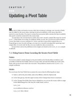
2. In the Name Manager, the Excel Tables and defined names are listed (see Figure 7-1).
Select a name in the list, and in the Refers To box, you’ll see the worksheet name on
which the range is located.
Figure 7-1. Name Manager dialog box
CHAPTER 7
■
UPDATING A PIVOT TABLE140
■
Tip
If the Refers To formula for a defined name contains #REF! errors, the worksheet, or some of its cells,
may have been deleted.
3. If errors are in the formula for a defined name, correct them if possible, or delete the
problem name, and then select a new source for the pivot table.
■
Note

The formulas for Excel Tables cannot be changed in the Name Manager. Close the Name Manager,
and then make the changes on the worksheet where the Excel Table is located. To add rows or columns,
drag the resize handle at the bottom right of the last cell in the Excel Table.
7.2. Using Source Data: Automatically Including New Data
Problem
Your pivot table is based on data in the same Excel file, and you frequently add new records to
the source data. Each time you add records, you have to change the source range for the pivot
table, to include the new rows.
You would like the source data range to automatically expand to include any new rows
and columns. This problem is based on the NewData.xlsx sample workbook.
Solution
When creating a pivot table from Excel data, the best solution is to create a formatted Excel
Table from the data, as described in Section 1.4. Then, use the name of the Excel Table as the
source for the pivot table. The Excel Table automatically adjusts if records are added or
deleted, and the pivot table includes the latest data when it’s refreshed.
If you don’t want to use a formatted Excel Table, you can use a dynamic range as the pivot
table’s source. The dynamic range automatically expands to include the new rows and
columns. Follow these steps to create a dynamic range, in the sample file:
1. On the Orders sheet, select cell A1, which is the top-left cell in the source range.
This step isn’t necessary, but it helps you by inserting the cell reference in the name
definition.
2. On the Ribbon, click the Formulas tab, and then in the Defined Names group, click
Define Name, to open the New Name dialog box.
3. In the Name box, type a name for the dynamic range, for example, PivotSource.
4. Leave the Scope setting as Workbook, and add a comment (optional), to describe the
name or its purpose.
CHAPTER 7
■
UPDATING A PIVOT TABLE 141
5. In the Refers To box, type an OFFSET formula that references the selected cell

=OFFSET(Orders!$A$1,0,0,COUNTA(Orders!$A:$A),COUNTA(Orders!$1:$1))
or you can use a nonvolatile formula, which may be more efficient in larger work-
books, where calculation speed is an issue:
= Orders!$A$1:INDEX(Orders!$1:$10000,
COUNTA(Orders!$A:$A),COUNTA(Orders!$1:$1))
The formula is set to a limit of 10,000 rows, which can be increased if required.
6. Click the OK button.
■
Caution
These formulas do not work correctly if other items are in Row 1 or Column A of the Orders
worksheet. Those items would be included in the count, and would falsely increase the size of the source
range, or they could cause an error when the pivot table is refreshed. Blank cells within the data in the row
or column being counted would also cause a problem, reducing the size of the source range. Count a column
and row where there is always a value.
After you create the named range, change the pivot table’s source to the dynamic range:
1. Select a cell in the pivot table, and on the Ribbon, click the Options tab.
2. In the Data group, click Change Data Source.
3. In the Table/Range box, type the name of the dynamic range, PivotSource in this
example, and then click OK.
■
Tip
While in the Table/Range box, delete the existing table or range. Then, to see a list of defined names,
press the F3 key. Click a name in the Paste Name dialog box, to select it, and then click OK.
How It Works
The OFFSET function returns a range reference of a specific size, offset from the starting range
by a specified number of rows and columns. The function has three required arguments
(shown in bold font), and two optional arguments:
=OFFSET(reference,rows,columns,height,width)
In our example
=OFFSET(Orders!$A$1,0,0,COUNTA(Orders!$A:$A),COUNTA(Orders!$1:$1))

CHAPTER 7
■
UPDATING A PIVOT TABLE142
the returned range starts in cell A1 on the worksheet named Orders. It is offset zero rows and
zero columns. The height of the range is determined by counting the cells that contain data
in Column A of the Orders worksheet:
COUNTA(Orders!$A:$A)
■
Note
If Column A contains any blank cells within the data range, use a column that does not contain
blank cells. Blank cells reduce the count and result in a range that is too small.
The width of the range is determined by counting the cells that contain data in Row 1 of
the Orders worksheet:
COUNTA(Orders!$1:$1)
This creates a dynamic range, because if rows or columns are added, the size of the range in
the defined name increases.
The INDEX formula is similar, but it creates a range that starts in Cell A1 on the Orders
sheet, and ends at the cell referenced by the INDEX function.
= Orders!$A$1:INDEX(Orders!$1:$10000,
COUNTA(Orders!$A:$A),COUNTA(Orders!$1:$1))
7.3. Using Source Data: Automatically Including New Data
in an External Data Range
Problem
In your workbook, you imported a text file that contains billing data, on to the BillingData
worksheet. This created an external data range that has a connection to the text file. If new
billing records are added to the external file, they appear in the external data range when it’s
refreshed. However, the pivot table is based on the imported data, but when you refresh the
pivot table, the new records don’t appear.
You can’t create a formatted Excel Table from the external data range, or the connection
to the external data will be lost.

This problem is based on the Billing.xlsx sample workbook. Depending on your secu-
rity settings, you may see a security warning when opening the sample file. To work with the
file, you can enable the data connections.
Solution
When you import external data to an Excel worksheet, using the commands in the Get Exter-
nal Data group on the Data tab of the Ribbon, a named External Data Range is created for the
imported data. If you base the pivot table on this named range, it expands automatically as
new records are added, and the pivot table contains all the data.
CHAPTER 7
■
UPDATING A PIVOT TABLE 143
When you created a pivot table from the external data, you may have used a reference to
range of cells, such as BillingData!$A$1:$J$19, instead of using the external data range’s name.
If data is added to the external data file, the new data appears in the Excel workbook, when the
external data range is refreshed. However, the pivot table continues to use the original range,
and the new data is not included in the pivot table when it’s refreshed.
Follow these steps to change the pivot table’s data source, so it uses the external data
range name:
1. To see the name of the external data range, right-click a cell in the external data range,
and then click Data Range Properties. The range name is shown at the top of the Exter-
nal Data Range Properties dialog box. Click OK to close the dialog box.
2. To base the pivot table on this range, select a cell in the pivot table, and then click the
Options tab on the Ribbon.
3. In the Data group, click Change Data Source.
4. Type the external data range’s sheet name and table name in the Table/Range box. For
example, if the sheet name is BillingData and the external data range name is Billing_1:
BillingData!Billing_1
5. Click OK.
7.4. Using Source Data: Moving the Source Excel Table
Problem

Your pivot table is based on a named range in another workbook. Using Windows Explorer,
you copied the two workbooks to your laptop, so you could work at home, but when you tried
to refresh the pivot table, you got an error message: “Cannot open PivotTable source file....”
This problem is based on the SalesData.xlsx and SalesPivot.xlsx sample workbooks.
Solution
You can reconnect the pivot table to the named range, in its new location:
1. Open both files—the file with the pivot table, and the file that contains the source data.
2. Activate the file that contains the pivot table, and then select a cell in the pivot table.
3. On the Ribbon, click the Options tab, and in the Data group, click Change Data Source.
4. While the Change PivotTable Data Source dialog box is open, on the Ribbon, click the
View tab. Click Switch Windows, and select the workbook that contains the source data.
5. Select the table that contains the source data, and then click OK.
■
Note
When you copy the files back to your desktop computer, you’ll have to follow the same steps to
reconnect them.
CHAPTER 7
■
UPDATING A PIVOT TABLE144