Event Order Abstraction for Parametric Real-Time System Verification pptx

Computer Science and Artificial Intelligence Laboratory
Technical Report
massachusetts institute of technology, cambridge, ma 02139 usa — www.csail.mit.edu
MIT-CSAIL-TR-2008-048 October 19, 2008
Event Order Abstraction for Parametric
Real-Time System Verification
Shinya Umeno
Event Order Abstraction for
Parametric Real-Time System Verification
∗
Shinya Umeno
Computer Science and Artificial Intelligence Laboratory,
Massachusetts Institute of Technology,
32 Vassar St, Cambridge MA, 02139, USA
Abstract
We present a new abstraction technique, event order abstraction (EOA), for parametric safety verification of
real-time systems in which “correct orderings of events” needed for system correctness are maintained by timing
constraints on the systems’ behavior. By using EOA, one can separate the task of verifying a real-time system
into two parts: 1. Safety property verification of the system given that only correct event orderings occur; and 2.
Derivation of timing parameter constraints for correct orderings of events in the system.
The user first identifies a candidate set of bad event orders. Then, by using ordinary untimed model-checking,
the user examines whether a discretized system model in which all timing constraints are abstracted away satisfies
a desirable safety property under the assumption that the identified bad event orders occur in no system execution.
The user uses counterexamples obtained from the model-checker to identify additional bad event orders, and
repeats the process until the model-checking succeeds. In this step, the user obtains a sufficient set of bad event
orders that must be excluded by timing synthesis for system correctness.
Next, the algorithm presented in the paper automatically derives a set of timing parameter constraints under
which the system does not exhibit the identified bad event orderings. From this step combined with the untimed
model-checking step, the user obtains a sufficient set of timing parameter constraints under which the system
executes correctly with respect to a given safety property.
We illustrate the use of EOA with a train-gate example inspired by the general railroad crossing problem [13].

We also summarize three other case studies, a biphase mark protocol, the IEEE 1394 root contention protocol,
and the Fischer mutual exclusion algorithm.
1 Introduction
In a typical real-time system, timing constraints on the system’s behavior are used to ensure its correctness. Such
a system is often modeled by using a set of timing parameters, rather than using concrete timing constants (for
example, [25, 27, 13]). These parameters specify, for instance, bounds on the duration between two specific events
in a system execution or certain delays, such as message delivery times.
Typically, only a subset of possible parameter combinations in the entire parameter space satisfies correctness
of such a system. A verification engineer or researcher typically follows one of the following two approaches to
formally verify such a system: 1. (Fixed-parameter verification) By fixing all timing parameters in the system,
he/she reduces the system model to a more tractable one such as an Alur-Dill timed automaton [1] and model-
checks the reduced system (using UPPAAL [20] or KRONOS [33], for instance [12, 6, 22]); or 2. (Parametric
verification) he/she treats the timing parameters as uninterpreted constants, finds an appropriate set of constraints
for the parameters, and manually proves or mechanically checks correctness under the constraints [25, 31, 34].
The second approach is attractive in the sense that if we can obtain a positive verification result by this approach,
then we have a concrete set of constraints on the timing parameters for the system to be correct, and may give an
implementation engineer more freedom of choice, than fixed-parameter verification.
The user can experiment with several instances of the first verification approach using multiple parameter
combinations, and then can try to figure out possible correlations between parameters in order for the system to be
∗
This work is supported by NSF Award 0702670. The conference version of this report will appear in proceedings of EMSOFT 2008 [30].
1
correct (for example, [27] uses this approach). However, these experiments by themselves never become exhaustive
if the number of possible parameter combinations is infinite (for example, a parameter can be real-valued, or an
integer but unbounded). Thus we need a more intelligent approach for completely parametric verification.
Another important challenge, in addition to time-parametric verification, is timing synthesis of a time-parametric
model. For timing synthesis, one tries to derive, in a systematic way, a sufficient set of timing parameter constraints
under which the system executes correctly. Automatic timing synthesis is considered to be an even harder problem
than automatic time-parametric verification since an algorithm or a tool is not a priori given a set of timing con-
straints by the user, but has to derive constraints by itself. A classical undecidability result about parametric timed

automata by Alur et al. [2] implies that a completely automatic timing synthesis does not terminate in general.
In this paper, we present a new abstraction technique, event order abstraction (EOA), for parametric safety ver-
ification of the subclass of real-time systems in which correct orderings of events maintained by timing constraints
on the systems’ behavior are critical for correctness (for example, a biphase mark protocol [25], the Fischer mutual
exclusion algorithm ([21], Section 24.2), and the IEEE 1394 root contention protocol [27]). By using EOA, one
can separate the task of verifying a safety property of a system into two parts: 1. Safety property verification of the
system given that only correct event orderings occur; and 2. Derivation of timing parameter constraints for correct
orderings of events in the system.
To use EOA, the user models a real-time system by using the time-interval automata (TIA) framework, which
is an extension of the I/O automata framework [21], and can express certain restricted class of timed I/O automata
[19]. By using the TIA framework, the user can specify lower and upper bounds on the time interval between a
specific event and a set of possible events that follow. The framework has a certain structure that is suitable for a
mechanical timing constraint derivation scheme presented in this paper.
A parametric verification of a real-time system using EOA is conducted in the following steps. First step is
identification of “bad” event orders. The user proposes a candidate set of bad event orders that he/she wants to
exclude from the system executions by timing synthesis. The user then model-checks a safety property of interest
on a discretized model of the underlying TIA, under the assumption that the model does not exhibit the proposed
bad event orders A discretized model of a TIA is simply an ordinary untimed I/O automaton that does not have
any timing constraints as the original TIA does. If the model-checking is completed with a positive answer, the
user has obtained a set of bad event orders that he/she needs to exclude. Otherwise, the user uses counterexamples
obtained from the model-checking to extract additional bad event order, and repeats the same process until he/she
successfully model-checks the discretized model.
The user expresses bad event orders by a simple language that can express a sequential order of events and some
types of repetition of events. He/she typically needs to apply human insight to extract from the counterexample a
bad event order expressed in a concise way, and this is why we have manually identified bad event orders for the
case studies presented in the paper.
Model-checking under a specific event order assumption can be carried out in the following two steps. The user
first constructs a monitor that raises a flag when one of the identified bad event orders is exhibited. Then he/she
model-checks the discretized model with this monitor under the assumption that the monitor does not raises a flag
(in Linear Temporal Logic (LTL) [23], this condition can be represented by: (¬Monitor.flag) ⇒

(¬DiscretizedMo del.propertyViolated)). We used the SAL model-cheker [9] in this paper. We manually con-
structed monitors since the construction was straightforward for the presented case studies (we are planning to
develop an automatic monitor construction tool). Since we successively refine the underlying discretized model
(by refining the bad order assumption) from a counterexample obtained from model-checking, EOA can be re-
garded as a counterexample guided abstraction refinement (CEGAR) technique [7].
Next, by an algorithm that we present in the paper, the user automatically derives timing parameter constraints
under which the system exhibits none of the identified bad event orders. From this step, the user obtains sufficient
timing constraints under which the system executes correctly with respect to a given safety property.
Related work: Some of the existing timed model-checkers (HYTECH [14], RED [32], TReX [3], LPMC [28], and
an extension of UPPAAL [18]) allow automatic synthesis of timing parameters for a specified desirable property of
a given system: these tools automatically derive a set of constraints on timing parameters for the system to satisfy
a given property. However, termination is in general not guaranteed for these model-checkers.
The main differences of EOA from the existing automatic timed model-checkers listed above are the following
four.
First, to use EOA, the user has to provide a set of bad event orders to be excluded in the system by timing
synthesis. Timed model-checkers mentioned above does not need such inputs.
2
Second, EOA can treat a class of systems that may exhibit an unbounded number of repetitions of events.
The existing parametric model-checkers listed above use symbolic reachability analysis of states symbolically
represented by linear logic expressions. Thus, if an underlying parametric model has an unbounded loop that
involves evolution of continuous variables, then this reachability analysis does not terminate, and therefore the
verification attempt fails (for example, in [14], Section 4.2, the authors stated that they had to modify a model
of a biphase mark protocol so that it exhibits no unbounded loop). In EOA, by using a language construct that
represents an unbounded number of repetitions of events, the user can handle this kind of system.
Third, when doing successive refinements by using EOA, each abstraction in a refinement step is a completely
untimed transition system (an ordinary I/O automaton with ordering constraints). Thus the user can directly employ
existing verification techniques for untimed transition systems.
Fourth, EOA does not suffer from the “dimensionality problem” as much as the timed model-checkers listed
above do. Automatic timing synthesis using the above listed model-checkers rapidly becomes intractable as the
number of parameters grows ( [14], Section 5. Lessons learned). This problem is called the “dimensionality

problem”, and is regarded as one of the main bottle necks of the time-parametric model-checkers. With EOA,
timing synthesis is handled separately from model-checking – the tool derives timing parameter constraints from
identified event orders just with information about time bounds between events, and does not use any information
about the state transition structure of the system. This synthesis process does not use a fixed-point computation as
timed model-checkers do, and thus does not need linear logic simplification for termination
1
. Instead, as we present
in Section 6, timing synthesis is done by a straightforward search within a certain space inferred by specified event
orders. In all case studies summarized in this paper, the search spaces were small. Indeed, the train-gate example
that we use to illustrate EOA throughout the paper has ten parameters, and the timing synthesis for it from specified
event orders took less than one second.
Frehse, Jha, and Krogh [11] presented a CEGAR-based approach for automatically synthesizing parameter
constraints of linear hybrid automata (LHA) [15]. Though this work is independently done from our work, the
approach is similar to ours in that it uses discrete abstraction of the underlying system to obtain counterexamples,
and then synthesize the timing (continuous) parameter constraints to exclude the obtained counterexamples. The
main differences between their approach and our approach are the following three: 1. Their approach automati-
cally identifies bad event sequences; 2: Their approach does not treat a repetition of events as our approach does
(Treating repetitions is crucial to verify certain examples such as the train-gate example in this paper and a biphase
mark protocol, for which meaningful parameter constraints can be obtained only by treating repetitive events);
3: Their approach treats LHA, which is more general than TIA. They experimented their approach by a simple
car-conflict prevention example, which has only two parameters. The applicability of their approach to a system
with a large number of parameters such as the ones in Section 7 is not known.
Several researchers considered digitization of timed transition systems [17, 5, 4, 26]. These techniques could
possibly be used to obtain a discrete version of real-time systems for fixed parameters, but as far as we know, an
application of the technique to parametric verification has not been studied.
We have developed EOA to fill in the gap between the inductive proof approach and automatic time-parametric
model-checking. The inductive proof approach needs human insights into an underlying system to come up with
an inductive property, and we believe that identifying bad event orders is more amenable process and requires less
training than coming up with inductive properties. On the other hand, automatic time-parametric model-checking
may not always scale to a system with a considerable number of timing variables and parameters, as we described

earlier.
When automatic time-parametric model-checker does not scale, one can try using inductive invariant reasoning
or by model-checking using parameter constraints as inputs – these are typically more scalable compared to auto-
matic parameter synthesis tools. To do so, he/she first needs to derive a set of timing parameter constraints under
which (he/she believes) the system works correctly. Typically the user performs this derivation by first drawing a
process communication diagram that depicts a possible bad scenario, and then manually finding out how to con-
strain timing parameters to exclude the depicted scenario. This approach is used in [31] to verify a biphase mark
protocol, and in [27] for the root contention resolving algorithm of the IEEE 1394 protocol. With EOA, the user
can directly make use of these human insights into the bad scenarios, and can also automate the process of deriving
timing constraints from the bad scenarios.
The rest of the paper is organized as follows. In Section 2, we introduce a new automata framework, time-
interval automata. We present the train-gate example, which is inspired by a railroad crossing problem [13],
1
Nevertheless, a linear logic simplification for a derived set of constraints is provided by the prototype tool for user’s convenience.
3
in the TIA setting. We use this example to illustrate the use of EOA throughout the paper. The example is
simple compared to an industrial protocol, for example, a biphase mark protocol that we study in Section 7,
yet has ten parameters and exhibits an unbounded repetition of events. In Section 3, we explain how the user
can formally specify event orders. In Section 4, we demonstrate how the user can conduct the bad-event-order
identification step. Section 5 is devoted to presenting the basis for automatic timing constraint derivation. In
Section 6, we present a prototype implementation that automatically synthesize timing constraint from given event
orders. Section 7 presents a detailed case study of time-parametric verification for the train-gate example using
EOA. We also summarize in Section 8 three other case studies, a biphase mark protocol that has been studied in
several verification papers (for example, [25, 31]), the IEEE 1394 root contention protocol [27], and the Fischer
mutual exclusion algorithm ([21], Section24.2). As a conclusion, in Section 9 we discuss a summary of the paper
and possible future work.
2 Time-Interval Automata
The time-interval automata (TIA) framework is an extension of the I/O automata (IOA) framework [21]. An I/O
automaton is a guarded-command style transition system with distinguished input, output, and internal actions.
Definition 1. (From [21]) An I/O automaton A (without a task partition) consists of four components:

• sig(A) = S, a signature, which is a triple consisting of three disjoint sets of actions: the input actions,
in(S), the output actions, out(S), and the internal action, int(S). We define the external actions, ext(S)
to be in(S) ∪ out(S); the locally controlled actions local(S), to be out(S) ∪ int(S); and act(S) to be all
the actions of S.
• states(A), a set of states
• start(A), a nonempty subset of states(A) known as the start states or initial states
• trans(A), a state-transition relation, where trans(A) ⊆ states(A) × acts(sig(A)) × states(A); we say
that action π is enabled in state s if there is a state s
′
such that (s, π, s
′
) ∈ trans(A). A must be input-
enabled, that is, in every state s, every input action π must be enabled.
Definition 2. An execution of an I/O automaton A is a (possibly infinite) sequence
α = s
0
, π
1
, s
1
, π
2
, · · · , π
r
, · · · where the s
i
’s are states of A and the π
i
’s are actions of A; s
0

∈ start(A); and for
any j ≥ 1, (s
j−1
, π
j
, s
j
) ∈ trans(A).
Informally, with the TIA framework, one can specify the lower and upper time bounds on the interval between
one action and its following actions for an underlying I/O automaton. A time bound for action a and actions in
B is represented as an interval in the form [l, u]. This bound represents that, for any time of occurrence t
a
of
action a, no action in B occurs before t
a
+ l, and at least one action in B is performed before or at t
a
+ u. An
interval-bound map defined in the following Definition 3 formally specifies this time bound. The special symbol
⊥ is used to express the time bound on the interval between the system start time and the time an action in the
specified set occurs.
Definition 3. (Internal-bound map). An interval-bound map b for an I/O automaton A is a pair of mappings, lower
and upper. Each of lower and upper is a partial function from actions(A)
⊥
× P(actions(A)) to R
>0
, where
actions(A)
⊥
= actions(A) ∪ {⊥} is a set of actions of A extended with a special symbol ⊥, P(actions(A)) is

the power set of actions of A, and R
>0
is the set of positive reals. We say that a time bound is defined for a pair
(π
⊥
, Π) ∈ actions(A)
⊥
× P(actions(A)) if either lower(π
⊥
, Π) or upper(π
⊥
, Π) is defined.
An interval-bound map defined in Definition 3 may not satisfy requirements to express a meaningful bound
(for example, the specified lower bound is no grater than the specified upper bound). Thus, we need a definition of
a valid interval-bound map (Definition 4).
Definition 4. A valid interval-bound map b for an I/O automaton A is an interval-bound map that satisfies the
following four conditions.
4
1. For every pair (π
⊥
, Π) ∈ actions(A)
⊥
× P(actions(A)), lower(π
⊥
, Π) and upper(π
⊥
, Π), if they are
defined, satisfy the following condition: 0 < lower(π
⊥
, Π) ≤ upper(π

⊥
, Π) < ∞.
2. For a pair (π
⊥
, Π) ∈ actions(A)
⊥
× P(actions(A)) with a time bound defined, Π ⊆ local(sig(A)).
3. For a pair (π, Π) ∈ actions(A) × P(actions(A)) with a time bound defined (note π is not ⊥), for any
(possibly infinite) subsequence β = π
r
s
r
π
r+1
· · · of an execution of A, if the following two conditions
hold, then at least one action in Π are enabled in any state that appears in β.
(a) π
r
= π.
(b) For all π
m
such that m > r and π
m
is in β, π
m
/∈ Π
4. For a pair (⊥, Π) ∈ {π} × P(actions(A)) with a time bound defined, for any (possibly infinite) prefix
β = s
0
π

1
s
1
π
2
· · · of an execution of A, if no action that appears in β is in Π, then at least one action in Π
are enabled in any state that appears in β.
The condition 1 states that the specified lower bound must be a finite real, and the lower bound must be less
than the upper bound. The condition 2 states that since we cannot control the timing of input actions (they are not
locally controlled), all timing-controlled actions must be local actions. The condition 3 guarantees that, for a pair
(π, Π) of an action and a set of actions with a bound defined, when the action π is performed, at least one action
in Π are enabled from then on until an action in Π is performed. The condition 4 is an equivalent of the condition
3 for the case of ⊥.
Definition 5. (Time-interval automaton). A time-interval automaton (A, b) is an I/O automaton A together with a
valid interval-bound map b for A.
Now we define how a time-interval automaton executes.
Definition 6. A timed execution of a time-interval automaton (A, b) is a (possibly infinite) sequence
α = s
0
, (π
1
, t
1
), s
1
, (π
2
, t
2
), · · · , (π

r
, t
r
), · · · where the s
i
’s are states of A, the π
i
’s are actions of A, and the t
i
’s
are times in R
≥0
; s
0
∈ start(A); and for any j ≥ 1, (s
j−1
, π
j
, s
j
) ∈ trans(A) and t
j
≤ t
j+1
.
We also require a timed execution to satisfy the lower and upper bound requirements expressed by b:
Upper bound:
1. For every pair of an action π and a set of actions Π with upper(π, Π) defined, and every occurrence of π
in the execution π
r

= π, if there exists k > r with t
k
> t
r
+ upper(π, Π), then there exists k
′
> r with
t
k
′
≤ t
r
+ upper(π, Π) and π
k
′
∈ Π.
2. For every pair of ⊥ and a set of actions Π with upper(⊥, Π) defined, if there exists k with t
k
> upper(⊥, Π),
then there exists k
′
with t
k
′
≤ upper(⊥, Π) and π
k
′
∈ Π.
Lower bound:
1. For every pair of an action π and a set of actions Π with lower(π, Π) defined, and every occurrence of π in

the execution π
r
= π, there does not exist k > r with t
k
< t
r
+ lower(π, Π) and π
k
∈ Π.
2. For every pair of ⊥ and a set of actions Π with lower(⊥, Π) defined, there does not exist k with t
k
<
lower(⊥, Π) and π
k
∈ Π.
The upper bound condition 1 states that if time ever passes beyond the specified upper bound for (π, Π) from
the time when π is performed, then an action in Π must occur in the interim. The lower bound condition 1 states
that, from any occurrence of π, no action in Π can occur before the specified lower bound. The second conditions
for upper bounds and lower bounds are analogous to the first conditions, but represents the requirement for bounds
with ⊥.
Definition 7. We say that a state s of a time-interval automaton (A, b) is reachable if there is a timed execution α
of (A, b) that ends with s.
In order to define a composition for time-interval automata, we need a definition of the compatibility of a
collection of time-interval automata.
5
Definition 8. For a finite collection of time-interval automata {(A
i
, b
i
)}

i∈I
, they are said to be compatible if the
underlying I/O automata {A
i
}
i∈I
are compatible, that is, for signatures S
i
and S
j
for A
i
and A
j
, respectively, if
i = j, then int(S
i
) ∩ acts(S
j
) = ∅ and out(S
i
) ∩ out(S
j
) = ∅.
Note that the “compatibility” of the bound maps {b
i
}
i∈I
(only one automaton can control timing behavior of
a specific action) is given by the compatibility for the automata signatures and timing controllability condition

(the condition 2 in Definition 4). That is, for any two pairs (π
i
, Φ
i
) ∈ actions(A
i
)
⊥
× P(actions(A
i
)) and
(π
j
, Φ
j
) ∈ actions(A
j
)
⊥
× P(actions(A
j
)), if time bound for both pairs are defined, then Φ
i
∩ Φ
j
= ∅.
Now we are ready to define a composition of time-interval automata.
Definition 9. For a compatible collection of timed-interval automata, the composition (A, b) = Π
i∈I
(A

i
, b
i
) is the
timed-interval automaton as follows. (1). A is the composition of the underlying I/O automata {A
i
}
i∈I
(which is
an ordinary asynchronous composition with synchronization of input and output actions with the same name [21]),
and (2). lower is given by taking union of {lower
i
}
i∈I
and upper is given by taking union of {upper
i
}
i∈I
(by
regarding partial functions as sets of ordered pairs).
Note that, due to the compatibility of the bound maps {b
i
}
i∈I
, both lower and upper in the composed automa-
ton are single-valued functions from actions(A)
⊥
× P(actions(A)) to R
>0
.

A TIA must satisfy some specific conditions in order to have reasonable timing constraints on it’s behavior.
Namely, every execution of a TIA must be extended to a time-diverging execution. The feasibility of a TIA in
Definition 10 formally defines these conditions.
Definition 10. We say that a TIA (A, b) is feasible if every finite timed execution
α = s
0
, (π
1
, t
1
), s
1
, (π
2
, t
2
), · · · , (π
r
, t
r
), s
r
of (A, b) can be extended to an infinite timed execution α
′
=
s
0
, (π
1
, t

1
), s
1
, (π
2
, t
2
), · · · , (π
r
, t
r
), s
r
, with sup
i≥0
{t
i
} = ∞ (and α
′
satisfies the conditions of a timed exe-
cution of (A, b), stated in Definition 6).
Definition 11. (Discretized TIA) Given a TIA (A, b), the discretized model of (A, b) is simply an underlying
ordinary untimed I/O automaton A.
The set of (untimed) executions of a TIA (A, b) (obtained by ignoring time stamps in timed executions) is
contained by the set of executions of its discretized model A, since A does not have any timing constraint. Thus,
if A satisfies a safety property under a certain event ordering assumption for its executions, then (A, b) also does
so under the same ordering assumption.
Related work of the time-interval automata framework: The timed I/O automata (TIOA) framework [19]
is a highly expressive framework with which the user can specify continuous evolution of analog variables by
using differential equations and inequalities, as well as specifying discrete state transitions as in an ordinary I/O

automaton. Indeed, any TIA can be expressed as a TIOA as well. However, a TIOA does not have an explicit
time bound structure like a time-interval bound map of a TIA, and thus information about time bound cannot
be easily handled by the scheme or the tool presented in the paper (a time lower bound needs to be embedded
in the precondition of an action, and an upper bound needs to be expressed by another construct, the stop-when
statement).
The MMT (time-constrained) automata framework [24] is closely related to the TIA framework. While a TIA
specifies time upper and lower bounds on the interval between an event and a set of events that follow, an MMT
automaton specifies time upper and lower bounds on the duration that an action in a specific set of actions called a
task stays enabled. When we define a TIA, for a pair (π, Π) of an action and an action set with a bound defined,
we impose constraints on the TIA so that at least one action in Π must be enabled after π and before an action in Π
is performed. If we impose the same constraint on an MMT automaton, we have a framework similar to TIA. The
timed transition system framework [16] is close to the MMT automata framework, in that the lower and upper time
bound on the duration that one transition is enabled can be specified. One main difference between TIA and these
two frameworks is that in TIA, the user can use different bounds for the same set of actions depending on which
action precedes it. We need this feature to model certain class of real-time systems like a biphase mark protocol
[31].
The Alur-Dill timed automata framework [1] is arguably the best known framework to model a real-time
system, and is the theoretical foundation for timed model-checkers like UPPAAL [20] and KRONOS [33]. This
framework can model only a system with fixed timing parameters, but not a time-parametric system.
The parametric timed automata (PTA) framework introduced in [2] is a time-parametric version of the Alur-
Dill timed automata framework. In a PTA, the user specifies lower and upper bounds on a time interval in which
6
——————————————–
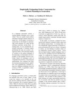
Automaton Train(r, R, p, P : Real) where
0 ≤ r ≤ R ∧ 0 ≤ p ≤ P
signature
output Request
output Pass
states
requested: Bool := false;

transitions
output Request
pre ¬requested
eff requested := true;
output Pass
eff requested := false;
bounds:
b(⊥, {Request}) = [r, R];
b(Pass, {Request}) = [r, R];
b(⊥, {Pass}) = [p, P ];
b(Pass, {Pass}) = [p, P ];
——————————————–
Figure 1: Train automaton
—————————————————————–
Automaton Gate(δ, ∆, τ, T, c, C: Real) where
0 ≤ δ ≤ ∆, 0 ≤ τ ≤ T , 0 ≤ c ≤ C
signature
input Request
output Close
output Open
output Check(result: Bool)
states
open: Bool := true;
train
requested: Bool := false;
check
succeeded: Bool := false
transitions
input Request
eff train

requested := true;
output Close
pre check
succeeded ∧ open
eff open := false;
output Open
pre ¬open
eff open := true;
train
requested := false;
check
succeeded := false;
output Check(result)
pre ¬check
succeeded ∧ result = train requested
eff check
succeeded := train requested;
bounds:
b(⊥, {Check(true), Check(false)}) = [δ, ∆];
b(Check(false), {Check(true), Check(false)}) = [δ, ∆];
b(Close, {Check(true), Check(false)} = [δ, ∆];
b(Check(true), {Close}) = [τ, T ];
b(Close, {Open}) = [c, C];
—————————————————————–
Figure 2: Gate automaton
the automaton stays in a specific location (in the Alur-Dill timed automata sense). A TIA can be modeled as a
PTA, but time bound for events becomes implicit (unlike the explicit interval-bound map) and thus cannot directly
use the automatic timing synthesis scheme presented in the paper.
Example 1. (Time-Interval Automaton). We describe an example of time-interval automata. The example is
inspired from railroad crossing problems [13]. The example is constructed from a composition of a train automaton

(Figure 1) and a gate automaton (Figure 2). An informal description of the problem we want to solve is the
following. A train is about to pass the railroad crossing with a gate. The gate is supposed to be open except for the
time that the train passes the crossing, so that cars can cross the railroad. When the train gets close to the crossing,
it requests to close the gate. The gate needs to be closed at the time the train passes the crossing. The railroad
actually forms a circle, and thus the train passes the railroad crossing cyclically. After the gate becomes closed, it
becomes open after a bounded time interval.
2
The actions of the Train automaton models actions taken by the train in the railroad. The Request action
represents an close request made by the train to the gate. The Pass action represents that the train passes the
crossing. The automaton has four bounds for these two actions. The first one (b(⊥, {Request}) = [r, R]) and the
second one (b(Pass, {Request}) = [r, R]) say that the Request action will be performed within the time interval
[r, R] after the system starts, and every time after the train passes the crossing, respectively. The third bound (b(⊥,
{Pass}) = [p, P]) and the forth bound (b(Pass, {Pass}) = [p, P ]) say that the Pass action will be performed within
the time interval [p, P ] after the system starts, and every time after the train passes the crossing, respectively.
3
The gate automaton described in Figure 2 models a gate system that uses a busy-wait loop for checking whether
a request has been made. The gate automaton cannot immediately know the arrival of an request. Instead, a
request information is stored in a state variable train
requested, and the gate automaton needs to repeatedly
2
If the reader prefers an example with more digital system flavor than the train-gate example, he/she can regard this example as, for instance, the following
single-writer/multi-reader shared variable problem: one writer process (Train) writes to a shared variable (railroad crossing) periodically, and before writing to the
variable, it first requests the guardian process (Gate) to lock the variable so that any reader (a car crossing the rail-road) cannot access to the variable while the
writer is writing to it.
3
We could, for example, think that a train is moving with a bounded velocity within [v
min
, v
max
], and the length of the railroad is L. The time bound of

[p, P ] for the pass event is equivalent to saying that p = L/v
max
and P = L/v
min
.
7
check this variable (expressed by a successful check, Check(true), and a failing check, Check(false)). We set the
time interval between two repeated checks to be within [δ, ∆]. Once a check succeeds, the gate automaton stops
checking train
requested, but resumes it within [δ, ∆] after the gate becomes closed. The gate becomes closed
(Close action) within the time interval [τ, T] after a successful check. The gate becomes open again (Open action)
withing the time interval [c, C] after it becomes closed.
The safety property that we want to verify is that the train passes the crossing only when the gate is closed.
We use a monitor automaton Monitor that monitors output actions Pass, Close, and Open from Train and Gate,
and set its state variable bad to true if Pass occurs when the gate is open. A formal description of the monitor
automaton is shown in Figure 3.
————————————–
Automaton Monitor
signature
input Pass
input Close
input Open
states
open: Bool := true;
bad: Bool := false;
transitions
input Pass
eff bad := if open
then true
else false;

input Close
eff open := false;
input Open
eff open := true;
————————————–
Figure 3: Monitor automaton
The invariant (safety property) we want to check is: for any reachable state of Train||Gate||Monitor, Moni-
tor.bad = false.
3 Specifying Event Orders
In this section, we introduce a formal way of specifying an event order that needs to be excluded for system correct-
ness. We first consider a simple way of specifying an event order, and then extend an event order specification by
introducing “don’t-care” events. The notion of these “don’t-care” events are important in order to treat a repetition
of events in a single system (as we will see in the case study for the train-gate example in Section 7) and in order
to ignore events by a process that is unrelated to a key local behavior in concurrent or distributed systems.
An event order (without “don’t-care”) simply specifies the order of consecutive actions in an execution of a
TIA. For example, the event order “Request-Pass” for the automaton (Train||Gate) shown in Example 1 matches
any execution of (Train||Gate) that contains a Request action immediately followed by a Pass action. We give a
formal definition of a match between an automaton execution and an event order in Definition 15, after introducing
“don’t-care” events. An event order may start with a ⊥ symbol, which specifies that the event order matches a
finite prefix of an execution of an underlying automaton. In other words, an event order that start with ⊥ specifies
the very first sequence of events that occur after the automaton starts executing.
Definition 12. (Event order) An event order of a time-interval automaton (A, b) is a sequence of actions of A,
possibly starts with a special symbol ⊥.
Example 2. (Event order). An example of event orders that we want to exclude in Train||Gate||Monitor discussed
in Example 1 is ⊥-Check(false)-Request-Check(true)-Pass. In this event order, the gate module first failed to
detect a request from the train since a request has not been made yet. After the train makes a request, the gate
module succeeds to detect it, and starts closing the gate. However, the gate close request is detected too late
8
relative to the speed of closing the gate, and consequently the train passes the crossing before the gate becomes
closed (that is, before the Close event occurs).

For a system that exhibits an unbounded repetition of events (such as the train-gate example in Example 1
and a biphase mark protocol that we study in Sections 7 and 8), some event orders to be excluded cannot be
represented in a form of a simple event order like the ones we consider earlier in this section. Consider the event
order “⊥-Pass” for (Train || Gate). This event order need to be excluded for an obvious reason: the train passes
the crossing even before the train requests that the gate be closed. Considering that the gate is doing a busy-
loop checking of a request, this Pass event can possibly be preceded by multiple failing checks (Check(false)).
Indeed, since the relation between the frequency of these checks (δ and ∆) and the time when a request is made
(r and R) is unknown, the number of possible failing checks that precede the Pass event is unbounded. What
we want to do is to ignore these failing checks in between ⊥ and Pass in the event order. By using a regular-
expression-like language, this event order can be expressed by “⊥-(Check(false))
∗
-Pass”, where ‘∗’ is a symbol
of repetition. The following event order using an ignored event specification (IES) is more comprehensible when
an event is ignored for a specific event-index interval, not just in between two consecutive events: E
2
= “⊥-Pass:
insert {Check(false)} to[0, 1]”. Informally, the ignored event specification (statement after insert)) in the above
event order E
2
specifies that when checking a match between an automaton execution and the event order, we
ignore in that execution any occurrence of Check(false) in between the beginning of the execution (e
0
) and the
first occurrence of Pass (e
1
). A formal definition of an IES is as follows.
Definition 13. (Ignored event specification). An ignored event specification (IES) for an event order is in the
following form: insert (Y
m
to [i

m
, j
m
])
r
m=1
, where Y
m
is a set of events that are ignored in the interval between
e
i
m
and e
j
m
.
To formally define a match between an automaton execution and an event order with an IES, we need I
E
k
that
represents the set of the ignored events in the interval between the k-th and (k+1)-st events in E (⊥ is considered
as the zero-th event).
Definition 14. (Ignored event set). For an event order with an IES,
E = (⊥)e
1
· · · e
n
: insert (Y
m
to [i

m
, j
m
])
r
m=1
, we define I
E
k
=

i
m
≤k<j
m
Y
m
for 0 ≤ k ≤ n − 1.
Definition 15. (Match between a timed execution and an event order with an IES). Consider a timed execution
α = s
0
, (π
1
, t
1
), s
1
, · · · of an time-interval automaton (A, b). Let α
′
be the sequence of actions that appear in α,

that is, α
′
= π
1
π
2
π
3
· · · . We say that α matches an event order with an IES,
E = e
1
· · · e
n
: insert (Y
m
to [i
m
, j
m
])
r
m=1
, if there exists a finite subsequence β of α
′
such that β can be split
into β
0
π
k
1

β
1
π
k
2
β
2
· · · β
n−1
π
k
n
, where, for all i, 1 ≤ i ≤ n, π
k
i
= e
i
, and β
i
is a sequence of actions and all
actions that appear in β
i
are in I
E
i
.
A match for an event order that starts with ⊥ is defined similarly to Definition 15 (an additional condition
k
1
= 1 is added to the definition). For an event order without an IES, all β

i
’s in Definition 15 are empty sequences.
We refer to an execution that matches E as E-matching execution.
4 Identifying Bad Event Orders
In this section, we illustrate how the user can extract bad event orders from counterexamples obtained from untimed
model-checking of the discretized model.
We use the train-gate example. The safety property we want to check is that the gate is closed whenever the
train passes the gate.
We first specified the following set of bad event orders as a candidate
4
:
A
1
. ⊥-Pass : insert {Check(false)} to [0, 1]
A
2
. ⊥-Request-Pass : insert {Check(false)} to [0, 1]
A
3
. ⊥-Request-Check(true)-Pass : insert {Check(false)} to [0, 1]
4
Of course, the user could instead start by model-checking the untimed model with no ordering constraint, and build up sufficient event orders. Nevertheless,
if the user knows partial information about what bad event orders might be, he/she can use human insight to set up a candidate set of bad orders at the beginning,
as in the presented case.
9
The above event orders A
1
, A
2
, and A

3
represent a situation that the train passes the crossing before the gate
becomes closed. A
1
specifies a situation that the train passes the gate even before it requests the gate be closed. A
2
specifies a situation that the train has requested the gate be closed, but the gate automaton does not detect a request
before the train passes the crossing. A
3
specifies the situation that the gate automaton successfully detects a close
request, but the gate does not become closed before the train passes the crossing. Here we used our human insight
into the underlying system that an unbounded number of Check(false) events can appear before the Request
event.
We manually constructed event order monitors, {EOM
i
}
3
i=1
, for these event orders, and then model-checked
the untimed model under the assumption that the above orders do not appear in system executions. In Linear Tem-
poral Logic (LTL) [23], this condition can be expressed by: UntimedTrain||UntimedGate||SM |=
(¬

3
i=1
EOM
i
.flag) ⇒ (¬SM.propertyViolated). A counterexample that can be obtained from a LTL expres-
sion in this form starts with a system execution that leads to a bad state, followed by a cycle in which the flags
of all monitors never become true. This is because we use the “always”  operator for the ordering assumption.

The user can basically ignore the cycle part and can just focus on the first part of the counterexample that contains
information about a bad event order.
When we model-checked the safety property with the ordering assumption that A
1
, A
2
, and A
3
do not occur,
we obtained the following counterexample execution: Request - Check(true) - Close - Open - Pass, followed by a
cycle in which

3
i=1
EOM
i
.flag never becomes true. This execution represents a situation that the gate successfully
becomes closed before the train passes the crossing, but becomes open again too fast. Since we knew that multiple
Check(false) events could have appeared before the Request event and after the Open event in this execution,
we identified the following bad event order.
B
1
. ⊥-Request-Check(true)-Close-Open-Pass : insert {Check(false)} to [0, 1], {Check(false)} to [4, 5]
In this way, the user can continue identifying bad event orders using both counterexamples from untimed
model-checking and human insight. We present the entire set of bad event orders for the train-gate example in
Section 7.
5 Deriving Timing Constraints
In this section, we present a scheme to derive a set of timing constraints to exclude an execution that matches a
given event order. The scheme just uses the bound map of an underlying TIA, but not the state-transition structure
of it.

Derivation of a timing parameter constraint for a given event order is taken in the following three steps:
1. We enumerate bounds on a pair of events in the event order that are immediately derivable from the bound
map b of an underlying TIA and the bound conditions in Definition 6.
2. We combine enumerated individual bounds to form a time bound for larger interval of events in order to
derive a meaningful constraint in the next step.
3. We find a matching pair of combined upper bound and lower bound, and then derive a timing constraint.
As we show in Section 6, this scheme forms the basis for the prototype implementation. More specifically,
each step of the above described scheme is systematic, and can be easily automated. We present a more detail of
each of the steps in the following.
Enumerating bounds: Given an event order E and the bound map b of a TIA, we first enumerate the upper and
lower bounds between the time of occurrence of two events in E from the upper and lower bound conditions in
Definition 6.
The following bound sets U
E
i,j
and L
E
i,j
contain upper and lower bounds between the times of occurrence of
the actions that match e
i
and e
j
in E, respectively, that are immediately derivable from the bound map b and the
upper and lower band conditions in Definition 6 (the ⊥ symbol is treated as the zero-th event e
0
). The bounds
are tagged with the event-index interval for which they are derived. Note that an upper bound for an event-index
interval [i, j] is constructed from the fact that a particular event does not appear in [i, j], whereas a lower bound
for [i, j] is constructed from the fact that particular events appear at i and j. This is consistent with the upper and

lower bound conditions in Definition 6.
Note that the bound map of an underlying TIA is used only in this first enumeration step.
10
Check(false) Request Check(true) Pass
Upper Bounds:
Lower Bounds:
∆
∆
δ
R
R
r
δ
T
p
δ
e1 e2 e3 e4(e0)
P
P
P
P
∆
(R,[0,1]) :
(R,[0,2]) :
(∆,[0,1]) :
(∆,[1,2]) :
(∆,[1,3]) :
(T,[3,4]) :
(P,[0,1]) :
(P,[0,2]) :

(P,[0,3]) :
(P,[0,4]) :
(δ,[0,1]) :
(r,[0,2]) :
(δ,[1,3]) :
(δ,[0,3]) :
(p,[0,4]) :
<
<
>
<
<
<
<
<
<
<
<
>
>
>
>
Figure 4: Upper and lower bounds for the event order E
1
For any E-matching execution α = s
0
(π
1
, t
1

)s
1
· · · , the matched subsequence of actions β = β
0
π
k
1
β
1
· · · β
k
n−1
π
k
n
(in Definition 15) satisfies t
k
j
− t
k
i
≤ u for (u, [i, j]) ∈ U
E
i,j
, and t
k
j
− t
k
i

≥ l for (l, [i, j]) ∈ L
E
i,j
. This fact is
proved as Lemma 1.
Definition 16. (Upper bound set). For i and j, 0 ≤ i < j ≤ n,
U
E
i,j
= {(u, [i, j]) | upper(e
i
, Π) is defined for some action set Π,
u = upper(e
i
, Π),
(j = i + 1 or e
i+1
· · · e
j−1
does not contain any action in Π), and
∪
j−1
k=i
I
E
k
does not contain any action in Π.}
Definition 17. (Lower bound set). For i and j, 0 ≤ i < j ≤ n,
L
E

i,j
= {(ℓ, [i, j]) | lower(e
i
, Π) is defined for some action set Π,
ℓ = lower(e
i
, Π), and e
j
∈ Π}
Lemma 1. For any E-matching timed execution α = s
0
(π
1
, t
1
)s
1
· · · , the matched subsequence of actions β =
β
0
π
k
1
β
1
· · · β
k
n−1
π
k

n
(in Definition 15) satisfies t
k
j
− t
k
i
≤ u for (u, [i, j]) ∈ U
E
i,j
, and t
k
j
− t
k
i
≥ l for
(l, [i, j]) ∈ L
E
i,j
.
Proof. By contradiction.
Upper bound set: Suppose t
k
j
− t
k
i
> u, or equivalently, t
k

j
> t
k
i
+ u. From the upper bound condition of a
timed execution stated in Definition 6, there exists k
′
> k
i
with t
k
′
≤ t
k
i
+ u and π
k
′
∈ Π. From the monotonicity
of the time increase, k
′
< k
j
. This contradicts the fact from the construction of (u, [i, j]) that, for any action
π
u
in Π for the upper bound definition upper(π, Π) = u from which (u, [i, j]) is derived, π
u
does not appear in
π

k
i
+1
· · · π
k
j
−1
.
Lower bound set: Suppose t
k
j
− t
k
i
< l, or equivalently, t
k
j
< t
k
i
+ l. From the lower bound condition of a timed
execution stated in Definition 6 and the construction of (l, [i, j]), there does not exist k > k
i
with t
k
< t
k
i
+ l and
π

k
∈ Π for the lower bound definition lower(π, Π) = l from which (l, [i, j]) is derived. This is a contradiction
since k
j
satisfies conditions for such a k.
Example 3. (Upper and lower bound sets). We show an example of U
E
i,j
and L
E
i,j
. The underlying automaton is
Train||Gate2||Monitor discussed in Example 1, the train-gate model with a busy-loop checking. As discussed in
Example 2, one of the event order that we want to exclude is E
1
= ⊥-Check(false)-Request-Check(true)-Pass.
Figure 4 depicts the upper bounds in U
E
1
i,j
and lower bounds in L
E
1
i,j
.
Upper bound example: We have an upper bound (R, [0, 1]) for the interval between e
0
(⊥) and e
1
(Check(false))

since we have an upper bound upper(⊥, {Request}) = R defined in the bound map, and the event Request is
not performed between e
0
and e
1
. For a similar reason, we have an upper bound (R, [0, 2]) between e
0
(⊥) and e
2
11
(Request). The upper bound set U
E
1
0,1
for the interval between e
0
and e
1
is: {(R, [0, 1]), (P, [0, 1]), (∆, [0, 1])}
Lower bound example: We have a lower bound (δ, [1, 3]) for the interval between e
1
(Check(false)) and e
3
(Check(true)) since we have a lower bound
lower(Check(false), {Check(false), Check(true)})) = δ defined in the bound map.
Combining bounds: We need a notion of a covering upper bound set and a distributed lower bound set to com-
bine individual bounds in U
i,j
and L
i,j

, respectively, so that we can synthesize a meaningful timing constraint.
Informally, a covering upper bound set U for an event interval Γ is a set of upper bounds such that when we take
a union of all intervals that tag upper bounds in U, the union becomes Γ (tagged intervals of upper bounds in U
cover Γ). A distributed lower bound set L for an event interval Γ is a set of lower bounds such that each interval
that tags a lower bound in L is contained in Γ, and all intervals that tag lower bounds in L do not overlap (tagged
intervals of lower bounds in L are distributed in Γ, without overlapping).
Definition 18. (Covering upper bound set). Consider a set of upper bounds S = {(u
k
, [i
k
, j
k
])}
m
k=1
for a time-
interval automaton (A, b) and an event order E (possibly with an IES), where (u
k
, [i
k
, j
k
]) ∈ U
E
i
k
,j
k
for k, 1 ≤
k ≤ m. We say that S covers the interval between e

v
and e
w
if for any event pointer p, v ≤ p ≤ w −1, there exists
an upper bound (u
k
1
, [i
k
1
, j
k
1
]) ∈ S such that i
k
1
≤ p and p + 1 ≤ j
k
1
.
Definition 19. (Distributed lower bound set). Consider a set of lower bounds S = {(l
k
, [i
k
, j
k
])}
m
k=1
for a time-

interval automaton (A, b) and an event order E (possibly with an IES), where (l
k
, [i
k
, j
k
]) ∈ L
E
i
k
,j
k
for k, 1 ≤ k ≤
m. We say that S is distributed in the interval between e
v
and e
w
if the following two conditions hold:
1. For any lower bound (l
k
1
, [i
k
1
, j
k
1
]) ∈ S, v ≤ i
k
1

and j
k
1
≤ w.
2. For any two lower bounds (l
k
1
, [i
k
1
, j
k
1
]), (l
k
2
, [i
k
2
, j
k
2
]) ∈ S, j
k
1
≤ i
k
2
or j
k

2
≤ i
k
1
.
Example 4. (A covering upper bound set and a distributed lower bound set). Let us look at Figure 4 again. The set
of upper bounds {(R, [0, 2]), (∆, [1, 3]), (T, [3, 4])} covers the interval between e
0
and e
4
([0, 2] ∪ [1, 3] ∪ [3, 4] =
[0, 4]). Each lower bound by itself constructs a lower bound set that is distributed in the interval between e
0
and
e
4
, but any set with two or more lower bounds is not distributed in the same interval, since we have some overlap
of the intervals for which the lower bounds are defined.
Deriving bounds: The following Theorem 2 implies that if we find a covering upper bound set and a distributed
lower bound set for the same interval, then we can obtain the timing constraints by the third condition in the
theorem (the sum of the upper bounds is strictly less than the sum of the lower bounds).
Theorem 2. Consider an event order E. A time-interval automaton (A, b) exhibits no E-matching execution if
there exists a set of upper bounds U = {(u
m
, [i
m
, j
m
])}
p

m=1
where (u
m
, [i
m
, j
m
]) ∈ U
E
i
m
,j
m
, a set of lower
bounds L = {(l
r
, [i
r
, j
r
])}
q
r=1
where (l
r
, [i
r
, j
r
]) ∈ L

E
i
r
,j
r
, and two events e
v
and e
w
such that the following three
conditions hold:
1. U covers the interval between e
v
and e
w
.
2. L is distributed in the interval between e
v
and e
w
.
3.

p
m=1
u
m
<

q

r=1
l
r
.
We need the following supporting lemmas (Lemmas 3 and 4) to prove Theorem 2.
Lemma 3. Consider a set of real-number intervals {[t
1
i
, t
2
i
]}
n
i=1
and an interval [t
1
, t
2
] that satisfies the following
two properties:
1. For each i, 1 ≤ i ≤ n, there is some real number u
i
such that t
1
i
− t
2
i
≤ u
i

.
2.

n
i=1
[t
1
i
, t
2
i
] = [t
1
, t
2
].
If such a set exists, then t
2
− t
1
≤

n
i=1
u
i
.
Proof.

n

i=1
[t
1
i
, t
2
i
] = [t
1
, t
2
] implies that

n
i=1
(t
2
i
−t
1
i
) ≥ t
2
−t
1
(otherwise the union of the underlying intervals

n
i=1
[t

1
i
, t
2
i
] cannot entirely cover the interval [t
1
, t
2
]). Since

n
i=1
(t
2
i
− t
1
i
) ≤

n
i=1
u
i
, the condition holds.
12
Lemma 4. Consider a set of real-number intervals {[t
1
i

, t
2
i
]}
n
i=1
and an interval [t
1
, t
2
] that satisfies the following
three properties:
1. For each i, 1 ≤ i ≤ n, there is some real number l
i
such that t
1
i
− t
2
i
≥ l
i
2. For any i, 1 ≤ i ≤ n, [t
1
i
, t
2
i
] ⊆ [t
1

, t
2
].
3. For any i and j, 1 ≤ i < j ≤ n, [t
1
i
, t
2
i
] ∩ [t
1
j
, t
2
j
] = ∅.
If such a set exists, then t
2
− t
1
≥

n
i=1
l
i
.
Proof. Since all intervals in {[t
1
i

, t
2
i
]}
n
i=1
are disjoint and are inside of [t
1
, t
2
],

n
i=1
(t
2
i
− t
1
i
) ≤ t
2
− t
1
(otherwise
there must be an overlap between some two intervals in {[t
1
i
, t
2

i
]}
n
i=1
). Since

n
i=1
(t
2
i
− t
1
i
) ≥

n
i=1
l
i
, the
condition holds.
Now we are ready to prove Theorem 2.
Proof. (of Theorem 2). By contradiction. Suppose the conditions for the theorem hold, but there is an E-matching
timed execution α = s
0
, (π
1
, t
1

) · · · . This implies that there is a subsequence of actions β = β
0
π
k
1
β
1
· · · β
k
n−1
π
k
n
that satisfies the conditions described in Definition 15. From Lemma 1, for each (u, [i
m
, j
m
]) ∈ U, t
k
j
m
− t
k
i
m
≤
u
m
holds, and for each (l
r

, [i
r
, j
r
]) ∈ L, t
k
j
r
− t
k
i
r
≥ l
r
holds. Since U covers the interval between e
v
and
e
w
, for any interval [t
d
, t
d+1
], u ≤ d ≤ v − 1, there is some u
m
∈ U such that [t
k
i
m
, t

k
j
m
] ⊇ [t
d
, t
d+1
]. Thus,

(u,[i
m
,j
m
])∈U
[t
k
i
m
, t
k
j
m
] = [t
u
, t
v
] Hence from Lemma 3, t
v
− t
u

≤

p
m=1
u
m
. On the other hand, since L is
distributed in the interval between e
v
and e
w
, [t
k
i
r
, t
k
j
r
] ⊆ [t
u
, t
v
] for any (l
r
, [i
r
, j
r
]), and for any two l

r
1 and l
r
2
∈ L, [t
k
i
r
1
, t
k
j
r
1
]∪[t
k
i
r
2
, t
k
j
r
2
] = ∅. Hence from Lemma 4, t
v
−t
u
≥


q
r=1
l
r
. Therefore,

q
r=1
l
r
<

p
m=1
u
m
.
This contradicts the third condition of the theorem assumption.
Example 5. (Timing constraint derivation for an event order without an IES). Again, consider the event order
depicted in Fig. 4. As discussed in Example 4, the upper bound set {(R, [0, 2]), (∆, [1, 3]), (T, [3, 4])} covers the
interval between e
0
and e
4
. In addition, the lower bound set {(p, [0, 4]} is distributed in the same interval. From
Theorem 2, if p > R + ∆ + T , then (Train || Gate2) exhibits no E
1
-matching execution.
Example 6. (Timing constraint derivation for an event order with an IES). Consider the event order E
2

= “⊥-
Pass: insert Check(false) to(0, 1)”. We have a lower bound lower(⊥, {Pass}) = p, and ⊥ appears at e
0
and Pass at e
1
. Thus we have a lower bound p between e
0
and e
1
(from Definition 17). We have an upper
bound upper(⊥, {Request}) = R defined for Train||Gate2, and the Request event is not ignored in the in-
terval between e
0
(⊥) and e
1
(Pass) – only Check(false) is ignored. Thus we have a valid upper bound R
between e
0
(⊥) and e
1
(Pass). Therefore, we can derive a constraint p > R, which imposes an order constraint
that a Request event must occur before a Pass event. On the other hand, though we have an upper bound
upper(⊥, {Check(true), Check(false)}) = ∆, we cannot derive an upper bound ∆ between e
0
and e
1
, since
Check(false) is ignored in that interval. Therefore, we cannot derive a constraint p > ∆. Indeed, the above
constraint does not exclude E
2

, since the constraint just imposes that the first Check event must occur before
Pass.
6 Implementation
We have implemented in Python a prototype of a timing constraint derivation tool (METEORS: MEchanical Tim-
ing / Event-ORder Synthesizer, version 0.1), based on the scheme described in Section 5. The problem that the
implemented prototype tool solves is as follows. The user gives the tool the set of time bounds defined in an under-
lying TIA for which he/she wants to derive a timing parameter constraint. Then the user gives the tool (typically
multiple) bad event orders to be excluded by timing synthesis. The tool first enumerates upper and lower bounds
immediately derivable from the given time bound information. The computational complexity of this enumeration
process grows only linearly with respect to the number of parameters (we need to do an enumeration for each pa-
rameter, and enumerations for different parameters are independent of each other). The tool then searches over all
possible covering upper bound sets and distributed lower bound sets. When the tool finds a matching pair of a cov-
ering upper bound and a distributed lower bound set, it derives timing constraints in the same way as demonstrated
in Examples 5 and 6.
13
The current prototype assumes both lower and upper bounds (p
i
and P
i
, respectively) are defined for all pairs
with bounds (π
i
, Π
i
) ∈ actions(A)
⊥
× P(actions(A)).
5
Therefore, the underlying TIA has the lower bound
parameter set {p

i
}
n
i=1
and the upper bound parameter set {P
i
}
n
i=1
, both of which contain the same number of
timing parameters, and a lower bound is at most as large as the matching upper bound: p
i
≤ P
i
.
A linear term over lower bound parameters {p
i
}
n
i=1
is in the form c
1
p
1
+ c
2
p
2
+ · · · + c
n

p
n
, which we also
write as

n
i=1
c
i
p
i
, where c
i
is an integer constant for 1 ≤ i ≤ n. A linear term over upper bound parameters
{P
i
}
n
i=1
is defined analogously.
An inequality the tool derives from one pair of a covering upper bound set and a distributed lower bound set
has the form φ > ψ, where φ =

n
i=1
c
i
p
i
is a linear term over lower bound parameters and ψ =


n
i=1
d
i
P
i
is a
linear term over upper bound parameters. The tool in general finds in a given event order multiple matching pairs
of covering upper bound sets and distributed lower bound sets, for each of which it can derive a linear inequality.
In such a case, multiple inequalities can be derived, and the given event order appears in no system execution if
at least one of the inequalities is satisfied. Thus, the tool derives a disjunction of linear inequalities for one given
event order.
The user typically needs to exclude multiple bad event orders. All specified event orders can be excluded if all
disjunctions of linear inequalities derived from the event orders are satisfied. Therefore, a timing constraint derived
by the tool forms a conjunction of disjunctions of linear inequalities – in a form similar to conjunctive normal form
of Boolean logic, but in our case we have linear inequalities instead of Boolean variables:

i∈I

j∈J
i
L
i,j
, where
L
i,j
is a linear inequality.
The constraint derived by the tool may first contain some unrealizable inequalities (for example, an upper bound
for a specific action set is strictly smaller than a lower bound for the same action set), or redundant inequalities

(for example, one inequality is weaker than or equivalent to another inequality in a disjunction). We use a simple
simplification algorithm to prune these inequalities, explained in the following.
6
We say that an inequality L appears as a solo inequality in a timing constraint (a conjunction of disjunctions of
linear inequalities)

i∈I

j∈J
i
L
i,j
, if there is a singleton set J
k
∈ {J
i
}
i∈I
, and

j∈J
k
L
i,j
is not a disjunction
of multiple inequalities, but simply the inequality L.
The tool finds out an unrealizable inequality by using the following fact. Given a linear term φ =

n
i=1

c
i
p
i
over lower bound parameters and a linear term ψ =

n
i=1
d
i
P
i
over upper bound parameters, if for all i, 1 ≤ i ≤ n:
c
i
≤ d
i
, then φ ≤ ψ. This is because p
i
≤ P
i
for 1 ≤ i ≤ n (the lower bound is at most as large as the upper
bound). Thus, for such a pair of φ and ψ, φ > ψ is not realizable. If the tool finds an unrealizable inequality, it
removes the inequality from a disjunction in the constraint.
A logical implication between two linear inequalities is also used to simplify the constraint. The tool makes
use of the following simple Lemma 5 to identify an implication.
Lemma 5. Suppose two linear terms φ
1
and φ
2

over lower bound parameters and two linear terms ψ
1
and ψ
2
over upper bound parameters have the following forms: φ
k
= Σ
n
i=1
c
k
i
p
i
; and ψ
k
= Σ
n
i=1
d
k
i
P
i
, for k = 1, 2.
Consider two linear inequalities (1) φ
1
> ψ
1
and (2) φ

2
> ψ
2
.
Inequality (1) implies Inequality (2) if for all i, 1 ≤ i ≤ n: c
1
i
− c
2
i
≤ d
1
i
− d
2
i
Proof. If we have φ
1
− φ
2
≤ φ
1
− φ
2
, then we are done since from (1), φ
1
− ψ
1
> 0, and thus (2) holds
from 0 < φ

1
− ψ
1
≤ φ
1
− φ
2
. Since p
i
≤ P
i
, (c
1
i
− c
2
i
)p
i
≤ (d
1
i
− d
2
i
)P
i
for all i, 1 ≤ i ≤ n. Therefore,
Σ
n

i=1
(c
1
i
−c
2
i
)p
i
≤ Σ
n
i=1
(d
1
i
−d
2
i
)P
i
, which is equivalent to φ
1
−φ
2
≤ ψ
1
−ψ
2
. Thus we have φ
1

−φ
2
≤ φ
1
−φ
2
,
as needed.
Now we explain how this implication-check scheme can be used to identify redundant disjunction of linear
inequalities in the constraint. The current prototype only focuses on a solo inequality in the constraint, since this
was sufficient to simplify the constraint for the four case studies we present in Sections 7 and 8.
Suppose we have a solo inequality A and a disjunction of inequalities B
1
∨ B
2
∨ · · · B
m
. If A implies B
i
for some i, 1 ≤ i ≤ m, then A ∧ (B
1
∨ B
2
∨ · · · B
m
) ≡ A. Therefore, if the tool finds in the constraint a solo
5
After obtaining a constraint simplified by the tool, the user can manually substitute p
i
= 0 for (π

i
, Π
i
) with only an upper bound, and can substitute
P
i
= ∞ for (π
i
, Π
i
) with only a lower bound. The current prototype does not make use of this information of “unbounded in one side” in a simplification of a
constraint, and this is our future work.
6
Note that this simplification process is completely independent of constraint derivation process, and is provided by the tool for user’s convenience. The
user could instead manually simplify the derived constraint or could use external linear-logic simplification tools as well. This is different from the timed/hybrid
model-checkers like HyTech, RED, TRex, and LPMC which inherently need an intelligent linear-logic simplification scheme to conduct a fixed-point calculation
for reachable states symbolically expressed by a linear logic expression.
14
inequality A and an inequality B in a disjunction D such that A implies B, then the tool can remove this whole
disjunction D from a constraint without changing the logical meaning of the constraint.
The tool uses an implication check to identify unrealizable inequalities as well. If the derived constraint in-
cludes a solo inequality φ > ψ, where φ =

n
i=1
c
i
p
i
and ψ =


n
i=1
d
i
P
i
, then the inequality E:

n
i=1
d
i
p
i
>

n
i=1
c
i
P
i
cannot be true for the constraint to be satisfied. Therefore, if one of the disjunctions in the constraint
includes an inequality that implies E, then this inequality cannot be satisfied, and thus can be removed without
changing logical meaning of the constraint.
Scalability experiment: To obtain a rough idea of the scalability of the constraint derivation process of the pro-
totype with respect to the event order length, we conducted an experiment on deriving a constraint for randomly
generated event orders of the train-gate example. This experiment (and all other experiments in this paper) was
conducted on a desktop computer with an Intel Core

TM
2 Quad at 2.66 GHz and 4GB memory. We experimented
with ten randomly generated event orders with length of thirteen, and the tool finished the constraint derivation
process within one second for all experiments. Considering that the length of the event orders that we identified for
the case studies presented in Sections 7 and 8 are all less than ten, the results of these experiments are satisfactory.
However, we have to conduct more case studies in order to examine the order of the length of the bad event orders
in larger real-time systems.
Discussion: Though the current prototype does not treat a “disjunctive” language construct (such as ∪ of a regular
expression), it is easy to derive a constraint for an event order that uses such a construct at the top level. For
example, suppose we want to exclude a (pseudo) event order e
1
e
2
{e
1
3
, e
1
3
}e
4
, which specifies that the third event
order is either e
1
3
or e
2
3
. We can simply treat this event order as two distinguished event orders e
1

e
2
e
1
3
e
4
and
e
1
e
2
e
2
3
e
4
.
Similarly, to exclude an execution that matches both of two event orders E
1
and E
2
(E
1
∩ E
2
in a regular
expression), we can individually derive constraints for E
1
and E

2
, and then disjunct them to obtain a constraint
(at least one of E1 and E
2
needs to be excluded to exclude E
1
∩ E
2
). Since we disjunct disjunctions of linear
inequalities derived for E
1
and E
2
, the derived constraint for E
1
∩ E
2
is a disjunction of linear inequalities. Thus,
derivation of a constraint from E
1
∩ E
2
(among other ordinary event orders) does not destruct the conjunction-of-
disjunctions structure of the final constraint.
7 Case Study: Train-Gate Problem
In this section, we illustrate the user of EOA and the prototype tool using the train-gate example Train||Gate||SM
that we have used in earlier sections of the paper.
We identified the following ten event orders to exclude all bad executions in the same way as described in
Section 4.
A

1
. ⊥-Pass : insert {Check(false)} to [0, 1]
A
2
. ⊥-Request-Pass : insert {Check(false)} to [0, 1]
A
3
. ⊥-Request-Check(true)-Pass : insert {Check(false)} to [0, 1]
A
4
. Pass-Open-Pass : insert {Check(false)} to [2, 3]
A
5
. Pass-Open-Request-Pass : insert {Check(false)} to [2, 3]
A
6
. Pass-Open-Request-Check(true)-Pass : insert {Check(false)} to [2, 3]
A
7
. Pass-Pass
B
1
. ⊥-Request-Check(true)-Close-Open-Pass : insert {Check(false)} to [0, 1], {Check(false)} to [4, 5]
B
2
. Pass-Open-Request-Check(true)-Close-Open-Pass : insert {Check(false)} to [2, 3], {Check(false)} to [6, 7]
C
1
. Close-Pass-Request
We can classify these event orders into three groups. The first group (A

1
- A
7
) represents a situation that the
train passes the crossing before the gate becomes closed. A
1
, A
2
, and A
2
are the event orders used as a first
candidate set of bad event orders in Section 4. In A
4
, A
5
, and A
6
, the ⊥ symbol in A
1
, A
2
, and A
3
, respectively, is
replaced by Pass-Open, so that they specify situations similar to A
1
, A
2
, and A
3

, but after at least one Pass events
have been performed. A
7
is like A
4
, but without Open after Pass. The second group (B
1
and B
2
) represents a
situation that the gate becomes open too fast after it becomes closed, and thus the gate is open when the train
passes the crossing. B
1
and B
2
intrinsically represents the same situation, but the ⊥ symbol in B
1
is replaced by
Pass-Open, so that B
2
specifies a situation after at least one Pass events have been performed. The third group
15
(C
1
) represents a situation that the gate becomes open again too late, that is, after the train makes a next request.
Since all state variables of the gate automaton are reset when the gate becomes open (by Open event), if the gate
becomes open after a request from the train, the request information is reset, and thus the gate would not become
closed.
In this bad order identification process, we manually constructed a monitor (a classical finite state machine) for
each of the identified ten event orders. Each monitor raises a flag exclude when it finds a subsequence of actions

that match the underlying event order in a current automaton execution. Actually, we could (manually) combine
some of the monitors
7
and needed to construct only six monitors (EOM1 - EOM6) at last. Model-checking for
each refinement step took less than one second. At the end of the bad order identification step, we successfully
model-checked the property (¬bad
event order) ⇒ (¬SM.propertyViolated) for
Train||Gate||SM||EOM1|| · · · ||EOM6, using a SAL symbolic model-checker [9], where bad event order =
EOM1.flag ∨ EOM2.flag ∨ · · · ∨ EOM6.flag.
For event orders A
2
, A
3
, A
5
, and A
6
, we had to do a “decomposition” of an event order. For example, we
cannot directly derive a meaningful constraint from A
3
. In A
3
, unlike the event order E
1
depicted in Figure 4,
we have possibly unbounded number of Check(false) events before Request, and these Check(false) events are
ignored. Thus, the bounds corresponding to (∆, [0, 1]), (∆, [1, 2]), (∆, [1, 3]), (δ, [0, 1]), and (δ, [1, 3]) in Figure 4
are removed from the set of enumerated bounds for deriving a constraint for A
3
, and therefore we cannot derive

the same constraint as in Example 5. Decomposing A
2
into the following two event orders resolved this problem:
one with no Check(false): A
′
3
= ⊥-Request-Check(true)-Pass, and one with one or more Check(false) events:
A
′′
3
= ⊥-Check(false)-Request-Check(true)-Pass :
insert {Check(false)} to [0, 1]. A
′′
3
still has an IES, but for this event order, an upper bound removed from the
upper bound set of E
1
in Figure 4 is only (∆, [0, 1]), and thus we can derive the same constraint p > R + T + ∆
as in Example 5. We decomposed A
3
, A
5
, and A
6
similarly to the case of A
2
described above. We manually
decomposed event orders for this case study, and automation of this decomposition is future work. More detailed
analysis and automation of this decomposition process is our future work.
After the decompositions of A

2
, A
3
, A
5
, and A
6
, we had fourteen event orders, and the tool derived the
following set of constraints from the given event orders after automatic simplification (the total time of derivation
and simplification took less than one second): 1. (p > R + T + ∆); 2. (r + t + c > P ∨ δ + t + c > P ); and
3. (r > C). The tool indicated that the first constraint was originally derived from a decomposed A
6
, the second
from B
1
, and the third from C
1
. Therefore, we obtained a constraint for each of the three groups we explained
above.
8 Summary of Other Case Studies
In this section, we summarize three case studies that we have conducted thus far. The case studies are: a biphase
mark protocol [25], the IEEE 1394 root contention protocol [27], and the Fischer mutual exclusion protocol ([21],
Section 24.2).
8.1 Biphase Mark Protocol
A biphase mark protocol [25] is a lower-layer communication protocol for consumer electronics. Several re-
searchers have conducted formal verification of this protocol (for example, [25, 31]), but as far as we know, com-
pletely automatic verification of it has not been done. We identified 22 bad event orders. (We successfully model-
checked the discretized model under the condition that 22 bad event orders do not occur, and model-checking
for each refinement step took less than one second). This number may look large, but similarly to the train-gate
example in Section 7, we identified multiple event orders from a single bad situation (there were eight bad situ-

ations). Eight event orders (derived from three situations) had to be decomposed as in the case of the train-gate
example. The tool derived five constraints (it took less than one second). Three of them are equivalent to the three
conditions manually derived in [31]. The remaining two constraints are not reported in [31], but we believe that
the constraint must hold for correctness (it is needed to exclude a simple bad scenario). In [31], the authors added
an additional condition during the verification process since they could not prove one key lemma. It seemed to
7
For example, by changing the initial state of the monitor for A
4
, we could also treat A
1
. Same for the pairs of A
2
and A
5
; A
3
and A
6
; and B
1
and B
2
.
16
us that this condition actually contradicts one of the three conditions they manually derived and assumed in the
verification process. A more detailed report on this case study will appear in a forthcoming publication [29].
8.2 IEEE 1394 Root Contention Protocol
The IEEE 1394 standard specifies communication infrastructure between electric devices. By using IEEE 1394,
up to 63 devices can be connected in a tree topology. The root contention protocol (RCP) that we studied is used at
the last phase of the tree topology identification. Though the bad scenarios to be excluded are two, due to the inter-

leaved process actions (events), we ended up having 42 event orders. The model-checking successfully completed
under the ordering assumption within one second. The tool derived a set of constraints that are equivalent to those
manually derived in [27]. A more detailed report on this case study will appear in a forthcoming publication [29].
8.3 Fischer Mutual Exclusion
The Fischer mutual exclusion algorithm ([21], Section 24.2) is a mutual exclusion algorithm that uses a timing
behavior for correctness. We identified one bad event order, by using the symmetry among process behavior.
In this event order, we focus on a specific interleaving of events between a pair of processes. Ignored event
specifications are used to treat behavior of other processes than the focused pair as “don’t-care”. We successfully
model-checked the discrete model under the correct ordering assumption (it took 40 seconds for a system with five
processes). The tool derived the constraint that is manually derived in [21].
9 Conclusion and Future Work
In this paper, we presented the event order abstraction (EOA) technique to parametrically verify real-time systems.
By using EOA, the user can directly make use of his/her intuition about what kind of bad scenarios need to be
prevented, by specifying bad event orders. We demonstrated the applicability of the technique by a simple train-
gate system and a summary of three other case studies, a biphase mark protocol, the root contention protocol of
IEEE 1394, and the Fisher mutual exclusion algorithm, are briefly reported.
This technique can be extended by enhancing automation of verification using EOA in the following processes:
construction of an event order monitor, decomposition of an event order, and extraction of a bad event order using
heuristics. An interesting future direction is extending bad event order language to treat a partial order of events,
as well as the current sequential order.
We consider that identifying bad event orders is useful not only for the verification/synthesis process of EOA,
but also for implementation engineers to understand what kind of undesirable scenarios can occur in the underlying
system/protocol when parameters are badly tuned. Along this line, identified bad event orders could be used in
model-based testing or model-based test-case generation [10, 8], in which a formally specified model is used to
test an actual implementation of a system.
Acknowledgment: First of all, I thank my supervisor, Prof. Nancy Lynch, for her patient guidance on this research
and fruitful comments on an earlier version of the paper. Also, several comments from Eunsuk Kang helped me
revise the paper. I also thank anonymous reviewers of a conference version of this paper for their helpful comments.
References
[1] Rajeev Alur and David L. Dill. A theory of timed automata. Theoretical Computer Science, 126(2):183–235,

1994.
[2] Rajeev Alur, Thomas A. Henzinger, and Moshe Y. Vardi. Parametric real-time reasoning. In ACM Symposium
on Theory of Computing, pages 592–601, 1993.
[3] Aurore Annichini, Ahmed Bouajjani, and Mihaela Sighireanu. TReX: A tool for reachability analysis of
complex systems. In Computer Aided Verification, pages 368–372, 2001.
17
[4] Eugene Asarin, Oded Maler, and Amir Pnueli. On discretization of delays in timed automata and digital
circuits. In Proc. of CONCUR’98, volume 1466 of Lecture Notes in Computer Science, pages 470–484, Nice,
France, 1998. Springer.
[5] Dragan Bosnacki. Digitization of timed automata. In Proc. of FMICS 99, 1999.
[6] Howard Bowman, Giorgio Faconti, Joost-Pieter Katoen, Diego Latella, and Mieke Massink. Automatic
verification of a lip-synchronisation protocol using uppaal. Formal Aspects of Computing, 10(5-6):550–575,
1998.
[7] Edmund M. Clarke, Orna Grumberg, Somesh Jha, Yuan Lu, and Helmut Veith. Counterexample-guided
abstraction refinement. In CAV 2000, volume 1855 of Lecture Notes in Computer Science, pages 154–169.
Springer, 2000.
[8] Siddhartha R. Dalal, Ashish Jain, Nachimuthu Karunanithi, J. M. Leaton, Christopher M. Lott, Gardner C.
Patton, and Bruce M. Horowitz. Model-based testing in practice. In International Conference on Software
Engineering, pages 285–294, 1999.
[9] Leonardo Mendonc¸a de Moura, Sam Owre, Harald Rueß, John M. Rushby, Natarajan Shankar, Maria Sorea,
and Ashish Tiwari. SAL 2. In Proc. of CAV 2004, volume 3114 of Lecture Notes in Computer Science, pages
496–500. Springer, 2004.
[10] Jeremy Dick and Alain Faivre. Automating the generation and sequencing of test cases from model-based
specifications. In FME ’93: Proceedings of the First International Symposium of Formal Methods Europe on
Industrial-Strength Formal Methods, pages 268–284, London, UK, 1993. Springer-Verlag.
[11] Goran Frehse, Sumit Kumar Jha, and Bruce H. Krogh. A counterexample-guided approach to parameter
synthesis for linear hybrid automata. In HSCC 2008, volume 4981 of Lecture Notes in Computer Science,
pages 187–200. Springer, 2008.
[12] K. Havelund, A. Skou, K.G. Larsen, and K. Lund. Formal modeling and analysis of an audio/video proto-
col: an industrial case study using uppaal. In RTSS ’97: Proceedings of the 18th IEEE Real-Time Systems

Symposium (RTSS ’97), page 2, Washington, DC, USA, 1997. IEEE Computer Society.
[13] C. Heitmeyer and N. Lynch. The generalized railroad crossing: A case study in formal verification of real-
time systems. Technical Report MIT/LCS/TM-511, MIT, 1994.
[14] T. Henzinger, J. Preussig, and H. Wong-Toi. Some lessons from the HYTECH experience. In Proc. of the
40th Annual Conference on Decision and Control, pages 2887–2892. IEEE Computer Society Press, 2001.
[15] T. A. Henzinger. The theory of hybrid automata. In LICS ’96: Proceedings of the 11th Annual IEEE
Symposium on Logic in Computer Science, page 278, Washington, DC, USA, 1996. IEEE Computer Society.
[16] Thomas A. Henzinger, Zohar Manna, and Amir Pnueli. Timed transition systems. In REX workshop Real-
Time: Theory in Practice, volume 600 of Lecture Notes in Computer Science, pages 226–251. Springer-
Verlag, 1992.
[17] Thomas A. Henzinger, Zohar Manna, and Amir Pnueli. What good are digital clocks? In Proc. of ICALP
1992, volume 623 of Lecture Notes in Computer Science, pages 545–558. Springer, 1992.
[18] Thomas Hune, Judi Romijn, Marielle Stoelinga, and Frits W. Vaandrager. Linear parametric model checking
of timed automata. In Tools and Algorithms for Construction and Analysis of Systems, pages 189–203, 2001.
[19] Dilsun K. Kaynar, Nancy Lynch, Roberto Segala, and Frits Vaandrager. The Theory of Timed I/O Automata.
Synthesis Lectures on Computer Science. Morgan & Claypool Publishers, 2006.
[20] Kim Guldstrand Larsen, Paul Pettersson, and Wang Yi. UPPAAL in a nutshell. International Journal on
Software Tools for Technology Transfer, 1(1-2):134–152, 1997.
[21] Nancy A. Lynch. Distributed Algorithms. Morgan Kaufmann Publishers Inc., 1996.
18
[22] O. Maler and S. Yovine. Hardware timing verification using kronos. iccsse, 00:23, 1996.
[23] Zohar Manna and Amir Pnueli. The Temporal Logic of Reactive and Concurent Systems: Specification.
Springer-Verlag, 1993.
[24] Michael Merritt, Francesmary Modugno, and Marc R. Tuttle. Time-constrained automata (extended abstract).
In Proc. of CONCUR 1991, volume 527 of Lecture Notes in Computer Science, pages 408–423. Springer,
1991.
[25] J Strother Moore. A formal model of asynchronous communication and its use in mechanically verifying a
biphase mark protocol. Formal Aspects of Computing, 6(1):60–91, 1994.
[26] Jo
¨

el Ouaknine and James Worrell. Revisiting digitization, robustness, and decidability for timed automata.
In Proc. of the 18th IEEE Symposium on Logic in Computer Science (LICS’03), pages 198–207, 2003.
[27] David P. L. Simons and Marielle Stoelinga. Mechanical verification of the IEEE 1394a root contention
protocol using Uppaal2k. International Journal on Software Tools for Technology Transfer, 3(4):469–485,
2001.
[28] RFL Spelberg and WJ Toetenel. Parametric real-time model checking using splitting trees. Nordic Journal
of Computing, 8:88–120, 2001.
[29] Shinya Umeno. Parametrically verifying embedded real-time protocols using event order abstraction. Tech-
nical report, Massachusetts Institute of Technology. To appear. (A conference version has been submitted for
publication).
[30] Shinya Umeno. Event order abstraction for parametric real-time system verification. In EMSOFT 2008:
International Conference on Embedded Software, August 2008. To apprear.
[31] Frits W. Vaandrager and Adriaan de Groot. Analysis of a biphase mark protocol with UPPAAL and PVS.
Formal Asp. Comput., 18(4):433–458, 2006.
[32] Farn Wang. Symbolic parametric safety analysis of linear hybrid systems with BDD-like data-structures.
Transactions on Software Engineering, 31:38–51, 2005.
[33] Sergio Yovine. KRONOS: a verification tool for real-time systems. International Journal on Software Tools
for Technology Transfer (STTT), 1(1-2):123–133, 1997.
[34] Dezhuang Zhang and Rance Cleaveland. Fast on-the-fly parametric real-time model checking. In Proceedings
of the 26th IEEE Real-Time Systems Symposium, pages 157–166, 2005.
19