Performance Modeling of Critical Event Management for Ubiquitous Computing Applications pptx
Bạn đang xem bản rút gọn của tài liệu. Xem và tải ngay bản đầy đủ của tài liệu tại đây (304.16 KB, 8 trang )
Performance Modeling of Critical Event Management for
Ubiquitous Computing Applications
Tridib Mukherjee, Krishna Venkatasubramanian, Sandeep K. S. Gupta
Department of Computer Science and Engineering
Arizona State University
Temp, AZ
tridib,kkv,sandeep.gupta @asu.edu
ABSTRACT
A generic theoretical framework for managing critical events in
ubiquitous computing systems is presented. The main idea is to
automatically respond to occurrences of critical events in the sys-
tem and mitigate them in a timely manner. This is different from
traditional fault-tolerance schemes, where fault management is per-
formed only after system failures. To model the critical event man-
agement, the concept of criticality, which characterizes the effects
of critical events in the system, is defined. Each criticality is asso-
ciated with a timing requirement, called its window-of-opportunity,
that needs to be fulfilled in taking mitigative actions to prevent sys-
tem failures. This is in addition to any application-level timing
requirements.
The criticality management framework analyzes the concept of
criticality in detail and provides conditions which need to be satis-
fied for a successful multiple criticality management in a system.
We have further simulated a criticality aware system and its results
conform to the expectations of the framework.
Categories and Subject Descriptors: C.4 [Performance of Sys-
tems]: Fault tolerance, Modeling techniques; C.4 [Special-Purpose
Application-based Systems]: Real-time and embedded systems; D.4.8
[Performance] Stochastic analysis; I.6.5 [Model Development]: Mod-
eling methodologies
General Terms: Performance, Reliability, Security, Theory.
Keywords: Autonomic Computing, Event Management, Proactive
Computing, Safety-Critical Systems, Ubiquitous Computing.
1. INTRODUCTION
Ubiquitous Computing (UC) systems (also known as Pervasive
Computing systems) [12] consist of a possibly large number of het-
erogeneous, massively distributed computing entities (e.g. embed-
ded wireless sensors, actuators, and various miniaturized comput-
ing and novel I/O devices), whose goal is to seamlessly provide
users with an information rich environment for conducting their
Supported in part by MediServe Information Systems, Consor-
tium for Embedded Systems and Intel Corporation.
Permission to make digital or hard copies of all or part of this work for
personal or classroom use is granted without fee provided that copies are
not made or distributed for profit or commercial advantage and that copies
bear this notice and the full citation on the first page. To copy otherwise, to
republish, to post on servers or to redistribute to lists, requires prior specific
permission and/or a fee.
MSWiM’06, October 2–6, 2006, Terromolinos, Spain.
Copyright 2006 ACM 1-59593-477-4/06/0010 $5.00.
day-to-day activities [1]. In order to provide effective services, in
such an environment, the UC system components need to be able
to interact seamlessly with one another. Any system, including UC
systems, broadly put, can be considered to be in one of the two
types of states - normal or abnormal. In a normal state, a system
provides services for routine events. For example - a smart hospi-
tal, responding to the arrival of critical patients may automatically
allocate appropriate resources such as available beds and contact
emergency personnel. These routine services may, however, be in-
adequate when the system is in an abnormal state. For example,
allocating resources when a natural disaster brings an influx of a
large number of patients to the hospital is a far more demanding
task. The changes in the system’s environment (external and/or in-
ternal) which lead the system into an abnormal state are called crit-
ical events (e.g. large influx of patient). The resulting effects, of
the critical events, on the system are called criticality (e.g. unable
to allocate resources for patients) [5].
Critical events and the consequent criticalities require unconven-
tional response from the system to be contained. For example, in a
disaster scenario, extra medical personnel may be brought in from
neighboring hospitals to manage the influx. We refer to such con-
tainment actions (e.g. response to a criticality) as mitigative actions
(e.g. bringing in extra medical staff) and the ability of handling crit-
ical events as manageability. Further, critical events usually have a
timing element associated with them requiring the system to con-
tain its effects within a certain amount of time. This is fundamen-
tally different from traditional systems, where any timing require-
ment is only provided by the application such as in real-time sys-
tems. Examples of timing requirement associated with criticalities
include - the golden
1
or critical hour
2
for many medical emergen-
cies such as heart attacks and diabetic coma and the mean-time
before shutting down a server/rack in a datacenter with a failed
cooling system is approximately few minutes (this depends upon
the specifics of a datacenter). We refer to this time period after the
occurrence of a critical event as its window-of-opportunity.
The criticality management process, to be effective and in order
to facilitate timely mitigative actions, has to detect critical events
as soon as they occur. This requires a level of proactivity, unlike
fault management in traditional systems, where fault tolerance is
exclusively employed in the event of faults. Even though, critical-
ity management is initiated in response to critical events, handling
them within their associated timing requirement, prevents the oc-
currence of system faults. For example - in the case of a datacenter,
the server racks (in the event of a failed cooling system) need to be
shut down within the datacenter dependent window-of-opportunity
hour (medicine)
Critical Hour
to prevent its failures. Criticality management therefore ensures
higher availability of the system by endeavoring to prevent failures.
Inclusion of timing constraints on mitigative actions makes crit-
icality aware systems look similar to real time systems. However,
there are some fundamental differences between the two. Real-
time systems intend to schedule a set of tasks such that they are
completed within their respective timing deadline. However, the
time to execute the tasks are fixed for the CPU where it would be
executed [9]. This is unlike the uncertainty involved, due to pos-
sible human involvement, in the time taken to perform mitigative
actions in response to critical events. Further, in real time systems,
completing tasks within their timing deadline guarantee successful
execution of jobs, whereas in case of criticality management, suc-
cessful completion of mitigative actions may not be deterministic
as it may also depend on the human behavior in response to crit-
ical events and the level of expertise in performing the mitigative
actions.
The contributions of this paper include a generic theoretical frame-
work for criticality management and the derivation of conditions
required for their effective manageability. This framework models
the manageability as a stochastic process by considering the vari-
ous states the system may possibly reach (as a result of criticalities)
and the probabilities of transitioning between them. The state tran-
sitions occur because of either new criticalities or mitigative actions
which take the system toward normality. To understand this frame-
work better, we simulated a criticality aware system by considering
three types of criticalities.
2. RELATED WORK
Ubiquitous systems are special type of embedded systems which
have been made possible by miniaturization of computing and com-
munication devices. Many embedded systems, e.g. heart pace-
maker and computer networks in modern cars, are safety-critical
systems [7]. Methodologies for designing and developing have
been well documented [4, 8]. This paper deals with ubiquitous
systems, which we refer to as criticality-aware systems, that fall
at the intersection of safety-critical systems, autonomic computing
systems (sharing the characteristics of self-manageability)
3
, and
proactive computing systems (sharing the characteristics of “deal-
ing with uncertainty”)
4
.
In recent years, development of relevant information technology
for disaster or crisis management is getting increasing attention
from teams of interdisciplinary researchers. A report from the Na-
tional Academy of Sciences [3] defines crises as “Crises,whether
natural disasters such as hurricanes or earthquakes, or human-made
disasters, such as terrorist attacks, are events with dramatic, some-
times catastrophic impact,” and “Crises are extreme events that
cause significant disruption and put lives and property at risk - situ-
ations distinct from “business as usual.”” In this paper, we refer to
these application-dependent crises as critical events and their effect
on a ubiquitous computing system as criticality.
The RESCUE project
5
is an interdisciplinary effort, which in-
volves computer scientists, engineers, social scientists and disaster
science experts, with the goal of developing information technol-
ogy for delivering “the right information to the right people at the
right time during crisis response.” This effort is focused on fast and
effective multimodal data gathering, analysis, dissemination and
presentation in a disaster situation [10]. The Secure-CITI project
6
www-03.ibm.com/autonomic/pdf/autonomic computing.pdf
www.intel.com/research/documents/proactivepdf.pdf
www.itr-rescue.org/.
www.cs.pitt.edu/s-citi.
is geared towards providing Emergency Managers for resource al-
location and decision making [11]. In contrast, this paper concen-
trates on modeling the entire criticality management system which
consists of physical, human, and virtual components. To the best
of our knowledge this is the first work towards the goal of identify-
ing crucial system parameters and properties, and determining the
necessary and sufficient conditions in terms of these parameters for
the system to satisfy these system properties.
The Caltech Infospheres Project
7
is focusing on “developing re-
liable distributed applications by composing software components
in structured way.” Applications of such compositional system -
“systems built from interacting components” - include any appli-
cation that requires “a sense-and-respond approach to data analysis
and problem solving, for instance, crisis management.” Ubiqui-
tous computing applications can be viewed as sense-and-respond
(S&R) systems. In [2], the author hints at evaluating S&R systems
in terms of timeliness and appropriateness of response (which we
refer to as mitigative actions).
In [5] the notion of criticality was presented informally and it
was applied to access control problem in smart spaces. Further, it
had a limited scope to manageability as it only addressed situations
with single criticality. Here, we take a more comprehensive and
formal approach and rigorously analyze the manageability of the
system when multiple simultaneous critical events occur. Exam-
ples of multiple criticalities in a system could include situations,
such as, massive patient influx in disasters (criticality 1) and lack
of required medical equipments (criticality 2) for treatment.
In [6], a game-theoretic based resource management system for
multi-crisis handling is presented. This work is mainly concerned
with strategies for expedited, fair (socially optimal) resource allo-
cation in multi-crisis situations in urban setting. Example of multi-
crisis scenarios includes an urban area with concurrently occurring
crisis events such as airplane crash at an airport, fight at a foot-
ball stadium, gas leak in a neighborhood, and multi-car accident
on a highway. The types of resources include fire trucks, police
units, and medical ambulances. As opposed to this work, this pa-
per focuses on generic performance modeling framework for such
systems.
3. SYSTEM MODEL
We define criticality in a criticality-aware ubiquitous system sys-
tem as follows:
Definition 1. Criticality is the effect on the system and its in-
habitants, as a result of events in the physical environment, which,
without timely mitigative actions involving possible human activi-
ties, would lead to loss of lives or properties.
Systems under one or more criticalities are said to be in a criti-
cal state. Criticality is associated with a time-constraint, called
the window-of-opportunity, that determines the delay between the
occurrence of the event causing the criticality and the resulting dis-
asters (such as loss of lives or properties). Events, that cause criti-
cality, are called the critical events. Any system in a critical state,
therefore, 1) has to detect and evaluate the severity of the critical
events, 2) plan and schedule appropriate mitigative actions accord-
ing to the available resources, 3) manage these actions to minimize
any uncertainty due to human involvement, and 4) impose these
actions to proactively avoid any disaster in the system. Figure 1
depicts the overall system with both physical and virtual compo-
nents. Criticality awareness in the virtual entities should be able to
effectively handle the criticalities and provide facilities for bringing
the system back to the normal state. However, improper evaluation
www.infospheres.caltech.edu/
Critical Events
Mitigative
actions
within
timing constraints
Normal State
Critical State
Disaster
State
Critical Events
Mitigative actions not
within timing constraints
Virtual
Entities
Physical Environment
Detection
Evaluation
Planning
Scheduling
Criticality
Awareness
Actuation
Figure 1: System components of an ubiquitous system and their interactions
of criticalities, mis-planning the mitigative actions, or missing the
timing requirements while scheduling these actions may fail to pre-
vent the disaster.
Let be the set of events in the physical environment and
be the set of critical events. The effects of event on the
system and its human inhabitants is denoted as criticality
. Let
be the set of all active (uncontrolled) criticalities in the system
when occurs. A criticality is active at any instance of time:
1. if the critical event has already occurred,
2. the mitigative action is not successfully performed till that
instance, and
3. the window-of-opportunity for the criticality is not over.
Each criticality is characterized by the 3-tuple ,
where
is the time when the critical event occurred,
is the window-of-opportunity for , and
is the set of possible mitigative (or corrective) actions for
in the system.
It is mandatory that any mitigative action in is performed within
in order to avoid disasters caused by the critical event .
The value of is not independent of other criticalities and is
also dependent on the human behavior in the physical environment.
Suppose models the probability of panic in the human inhab-
itants in the physical place at time ( ), in response to the
occurrence of event . Then, the value for criticality at time
can be given as where , for all ,
is a function over that defines the dependency of with other
active criticalities in the system and the resulting human behavior
as predicted. The average value of can therefore be obtained as
follows:
(1)
where is an upper bound for the window-of-opportunity. For
noncritical events,
tends to , thereby making undefined.
For critical events, however, this value is the best case value ob-
tained when there is no other active criticalities and the humans are
all trained to behave according to the situation. It should be noted
here that , where .
Each mitigative action , , is further character-
ized by the 4-tuple
, where:
is the average time taken to perform the action ,
is the set of resources that are required to perform the
action ,
is the average cost in performing , and
is the average probability of successful completion of
within for mitigating criticality .
The components that constitute the cost of mitigative action (
)
are application dependent parameters such as gathering certain re-
sources to perform the actions and error probability of the resources
under criticality
. If models the probability of error in
the mitigative action , due to human involvement, can be
represented as an application defined function over as follows:
(2)
where is the set of available resources (after the occurrence of
event ) and can be calculated as follows: if is the set of re-
sources at time , then . Further, due to
the involvement of human activities in the mitigative actions, the
successful completion of the actions is uncertain. Apart from this,
the unavailability of resources while performing the actions can
also lead to uncertain outcome of the mitigative actions (especially
in completing the action within the stipulated time). If is the
mitigative action enforced for mitigating criticality , then,
we can characterize the average probability of successful comple-
tion of , , by the following function over :
(3)
The probability of disaster i.e. the probability of loss of lives
or properties as a result of critical event can be given as
when mitigative action is employed.
4. FUNDAMENTAL PROBLEMS
Considering this model, the fundamental research questions that
are addressed in this paper are: 1) what are the basic principles for
the detection, evaluation and planning for criticalities?; and 2) how
to find the sequence of actions that either maximize the probabil-
ity of success and/or minimize the cost requirement in mitigating
the criticalities in the system. The window-of-opportunities for the
criticalities and the availability of resources in the system deter-
mine the constraints within which the objective has to be achieved.
Thus the problem can be formalized as follows:
(4)
where , The above problem intends to find the most cost-
effective mitigative actions for the critical events. The following
problem, however, intends to minimize the probability of disaster
due to critical events:
(5)
5. PROPERTIES OF CRITICALITY
This section identifies two generic properties for modeling crit-
icality aware systems: Responsiveness, and Correctness. Respon-
siveness measures the speed with which the system is able to ini-
tiate the detection of a critical event. Therefore, the higher the
responsiveness the more time there is to take corrective actions.
Correctness ensures that mitigative actions are executed only in
response to a critical event. Before we proceed to analyze these
properties, we make some simplifying assumptions about our sys-
tem model:
1. All criticalities are detected correctly, that is, their types and
properties are accurately known at the time of detection; and
2. We do not address malicious attacks on the detection process.
The modeling of accuracy of any event detection system involves
determination of probabilities of false positives and false negatives.
These are well-known and well-studied factors. Incorporation of
these probabilities, although important for overall modeling of the
system, would unnecessarily complicate the modeling in this pa-
per. Similarly, the uncertainty and problems introduced due to pres-
ence of malicious entities may be important for many applications.
However, we ignore this issue here and leave it for future work.
5.1 Responsiveness to Criticality
This section, presents an analysis of responsiveness to criticali-
ties in a system. It begin with analysis for the simple case of single
criticality in a system and then expands it to multiple criticalities.
5.1.1 Single Criticality
Responsiveness captures the fraction of time in
after which,
the corrective actions for a critical event are initiated. Upon occur-
rence of any critical event in the physical environment, the critical-
ity aware system should be able to detect the resulting criticality.
If is the time to process (evaluate the parameters of the critical
event and enforce mitigative actions) the detected event, then the
criticality can be controlled iff such that,
(6)
Further, has two main components:
1. the time to initiate the detection ( ), and
2. the time to process (identify the nature of the event) any de-
tected event ( ).
We characterize responsiveness with a term called Responsiveness
Factor (RF) which is defined as:
Definition 2. for all criticality .
Figure 2 shows the various states the system goes, over a timeline,
through while mitigating single criticality. In the first case, criti-
cality is not mitigated before the expiration of the . In the latter
case, criticality is mitigated successfully before expires. Higher
the RF for a criticality, lesser is the time (in terms of fraction of
window-of-opportunity) taken to respond to it. For successfully
handling of any criticality, the value of its RF must be greater than
1, otherwise, the time to respond to a critical event will be greater
than the total time available for it (limited by ).
We next define Utilization Factor as follows:
CE
T
CE
T
CE
T
p
i
i
p
Tend
Tstart
time
W
Tstart
start of time from system perspective
Tend
end of time from system perspective
occurrence of criticality
NORMAL
CRITICAL FAULTY
NORMAL
Ta
NORMAL
W
CRITICAL
Ta
Figure 2: Single Criticality Timing Diagram. Note that
and are depicted as and , respectively; and and
denote the duration of window-of-opportunity and the time
for performing the mitigative action for the single criticality,
respectively.
Definition 3. is the Utilization Factor for controlling
the criticality and is defined as the fraction of time taken (by ac-
tion
) for critical event processing and taking necessary
controlling actions in for criticality .
Responsiveness Condition
Replacing in Equation 6 with its constituents, we get
. Therefore,
(7)
Equation 7 is referred to as Responsiveness Condition for Sin-
gle criticality (RCS).
Equation 7 signifies that as the amount of time required to pro-
cess and control a criticality increases, the time available to initiate
its detection decreases, thereby imposing higher responsiveness re-
quirements. Therefore, in summary, the mitigation process has to
meet the RCS condition to prevent system faults.
5.1.2 Multiple Criticalities
In this section we generalize the above analysis for multiple crit-
icalities. In a system where multiple critical events have been expe-
rienced, mitigative actions cannot be taken in an arbitrary manner.
For example, in an hospital emergency department (ED), a patient
suddenly experiences a life-threatening ventricular fibrillation, may
require defibrillator treatment. If the defibrillator equipment sud-
denly malfunctions, then we have scenario with multiple criticali-
ties where we have to fix the defibrillator (through replacement or
repair) before treating the patient. This characteristic imposes a
priority over the handling process, where certain criticalities need
to be handled before certain others. Figure 3 illustrates a system
where multiple critical events have occurred. The criticalities are
mitigated according to their priority, thereby allowing the third crit-
icality, which occurred last, to be mitigated first and so on.
Controllability Condition
Let be a criticality which has occurred, and be the set
of (uncontrolled) critical events which have higher priority than .
Then,
can be controlled iff (in the worst case) for any ,
SECOND
CRITICALITY
THIRD
CRITICALITY
FIRST
CRITICALITY
TIME
DEFERRED
DEFERRED
MITIGATION
MITIGATION
THRID CRITICALITY
SECOND CRITICALITY
MITIGATED
MITIGATED
FIRST CRITICALITY
MITIGATED
PRIORITY
Figure 3: Multiple Criticalities
(8)
Here,
denotes the fraction of time, in , required for handling criticali-
ties with priorities higher than , thereby deferring the mitigation
of
. We refer to this as the Deference Factor (DF) for criticality
by the higher priority criticalities in ( ). There-
fore, Eq. 8 can be re-written as:
(9)
Equation 9 signifies the necessary and sufficient condition for
successfully handling any criticality in the system. Note that,
the condition is sufficient only for the case when the probability of
success for all mitigative actions is 1. In the case of single crit-
icality, the DF becomes 0, thereby degenerating equation 9 to 7.
We call the inequality in Equation 9 as Controllability Condition
( ) for any criticality . This condition acts as the constraint for
both the objective functions (Equations 4 and 5). In this paper, we
will only consider the objective function of Equation 5 (the same
methods can be applied to solve for the objective of Equation 4).
5.1.3 Periodicity of Detection
From the analysis of both single and multiple criticalities, it is
imperative that - to guarantee responsiveness, timely detection of
criticality is necessary. To achieve this, we need to periodically
monitor for critical events. This suggests the need for an auto-
matic (periodic) monitoring process which detects critical events
with the minimum possible delay. Detecting critical events, in
a non-automatic manner cannot guarantee a required responsive-
ness for the criticality, as the initiation of the detection process
can have any arbitrary amount of delay. To model the periodic-
ity of the criticality detection process, we designate , where
, as the period after which the
detection process is repeated. Here is a system dependent con-
stant which provides the lower bound for the detection initiation
period, and is the set of all possible criticalities. For a system
all possible criticalities are assumed to be known a priori, much
like exceptions in traditional systems.
5.2 Correctness of Criticality
Correctness ensures that any controlling steps are executed by a
system only in case of a critical event. This qualitative property
of criticality cannot be analytically modeled and depends on the
design and implementation of the system. For example, in a bank
1
2
N
1,1
1,2
1,1,1
1,2,1 1,2,2
2,1 2,N
2,1,1 2,1,2 2,N,N
N,1
N,N
N,1,1
2,N,N
p1
p2
p3
p4
p5
p6
p7
p8
p9
p’1
p’2
p’3
p’4
p’5
p’6
p’7
p’8
p’9
p’10
p’11
p’12
p’13
p’14
p’’1
p’’2
p’’3
p’’4
p’’5
p’’6
p10
p’’’2
p’’’1
p’’7
p’’8
p’’9
p’’10
p’’11
n
ABNORMAL STATES
Figure 4: Critical State Transition Diagram
environment, a criticality could be an unauthorized entry into the
vault. To detect this criticality and take mitigative actions (lock-
ing the exits, calling the law enforcement), the detection system
(hardware and software) has to work accurately, which is totally
dependent upon the hardware and software technologies used. The
probability distribution of accurately detecting a critical event de-
termines the probability of occurrence of the criticality in our sys-
tem. If, for example, the detection process is not very accurate
and reports a criticality even if there is no causing critical event,
the probability of occurrence of that critical event, in our system
analysis, becomes high.
6. MANAGEABILITY OF CRITICALITIES
In this section, we analyze the manageability of the critical events
as a stochastic process. The analysis presented here pertains to the
generalized case of multiple criticalities (single criticality manage-
ability being a trivial specialization). Further, in all the subsequent
analysis, we assume the maintenance of the correctness property.
Further, for the simplicity of notational representation, we have as-
sumed that for any
, only one action can be taken. The determi-
nation of which action to take from the set is trivial (the action
which has the highest that meets the condition).
6.1 Stochastic Model
When a criticality occurs in the system (in normal state), it moves
into the critical state (Figure 1). All subsequent criticalities keep
the system in the critical state. In order to model the handling of
multiple criticalities, we have to first express the critical state in
more detail. The critical state, as shown in Figure 1 encompasses
many system states which are reached in response to the occur-
rence of different criticalities. For example in Figure 4, state
is reached when the criticality occurs before successful handling
of criticality . The arcs between states represent the state tran-
sitions, each of which is associated with a probability value. State
transitions occur as a response to either critical events or mitiga-
tive actions. The state transition diagram is organized in a hierar-
chical format. Each occurrence of a criticality moves the system
down this hierarchy (the associated arc is called critical link (CL))
and each mitigative action moves it upward (the associated link is
called the mitigative link (ML)). The set of all CLs and MLs of any
node is referred as and , respectively. The proba-
bilities associated with a criticality link (an outgoing downward
arc) originating from a particular state represents the probability
of occurrence of the critical event associated with in state . On
the other hand, the probability associated with a mitigative link
(an outgoing upward arc) originating from a particular state rep-
resent the probability of successfully handling a criticality using
the mitigative action corresponding to link .
Let be the set of all criticalities which can occur in the sys-
tem. In Figure 4, initially the system is in the normal state. Now
suppose a criticality occurs, it will immediately move the
system into the state represented as . Before the system has a
chance to successfully mitigate the effects of , another criticality
occurs. This event will further move the system down the
hierarchy to the state represented by . Now in order for the
system to move up to the normal state it has to address (mitigate)
both criticalities before their respective window-of-opportunities.
The process of mitigation can be done in two ways in this case, by
mitigating criticality before or vice versa, the order of which
may be application and criticality dependent. Therefore, there are
potentially two paths in the hierarchy that the system can take to
reach the normal state. If both paths can be taken (the order of
criticality mitigation is immaterial), then the choice of the paths
depends upon two factors:
1. the probability of reaching the neighboring state (up the hi-
erarchy) from the current state, and
2. the average probabilities of success for reaching the normal
state from each of the neighbor state.
These average probabilities of success of reaching the normal state
from any neighbor state depends not only on the probabilities of
the MLs along the path but also on the possible criticalities (i.e
probabilities of the CLs) at the intermediate sates taking the system
down the hierarchy through CL. It should be noted that the sum of
probabilities for all outgoing state transition arcs from any state is
at most equal to 1, and the sum of probabilities of all outgoing CLs
from any state (denoted as
for state ) is less than 1.
As stated earlier we concentrate on objective function in Equa-
tion 5 which is concerned with finding a sequence of mitigative
actions (or next mitigative action) which minimizes the probabil-
ity of disaster (failure of the system to take appropriate corrective
actions.).
6.2 Minimizing Probability of Disaster
Consider the system which, as a result of multiple criticalities,
is in the state
(Figure 5). The goal is to find the path which has
the highest probability of success to reach the normal state (which
signifies the probability of mitigation for all the uncontrolled crit-
icalities). In order to do that, the system has to find a neighbor
state (up in the hierarchy) which has the highest probability of suc-
cessfully reaching the normal state
8
. Let state be any such neigh-
boring state. The probability of successfully reaching the normal
state(represented as state ) from state is given by a recursive
expression as follows,
&
where is the probability associated with the arc that goes from
state to state , is the average prob-
ability of criticality at state ,
is the average probability of reaching if no additional criticality
occurs at state , and is the av-
erage probability of reaching if an additional criticality occurs at
state . If the is not met for any state transition path
in the hierarchy then will be zero. Now, the probability of
success to reach from through neighbor state is given by:
We assume that once a criticality has been mitigated it does not occur again before
reaching the normal state.
i
X
j2
j3
j1
State transition paths to N via an intermediary state j*
n
Figure 5: Paths from State X to Normal State
0.2
0.1
0.3
0.2
0.1
0.5
0.7
0.4
n
a
b
x d
0.23
0.22
Figure 6: Example of State Transition Path
Therefore the best state to move to from state (in the pursuit
of reaching ) is the state (such that ) which
meets the following requirement:
.
The value is referred to as the Q-value for .
6.3 An Example
Consider a system with a state transition hierarchy as shown in
Figure 6. It represents a system which can have only two types of
criticalities ( and ). Further, assume that the system is currently
in the state and and for and are 10 and 20 units,
respectively. In this hierarchy, each ML has an associated
unit ( denotes the time required to take the mitigative
action of criticality that transits the system from to ). To find
the state transition path to from , we first individually compute
the average probability of success (of reaching ) from each of
the neighbors of state . In this example, the neighbors of state
are states and . The average probability of reaching from
is given (by applying Equation 10) as . This is
because, there is only one path from to and the system will
not move back from state to state . Further, we see that the
condition is met here because to move from to ( ) is 1
unit, making UF (when the system is at ). Also, as there are
no other criticalities, DF is 0, and is 0 (assuming instantaneous
initiation of detection). Therefore, the , which yields (0 + 0.1 +
0 10), holds true. Thus we have .
Similarly, the average probability of reaching state from state
is given by . It can further
be easily verified that is met if any path through (
, or ) is taken. The
above equation reduces to
. Now, the probability of success
in reaching from through and are
and . Therefore, the best way
to reach from is through state . However, if we set to be 2
units (instead of 20 units), then we have
as the path does not meet the
making to be 0.156. However as is still 0.161, the
path is now the better choice.
We next state an important theoretical result.
6.4 Manageability Theorem
The following theorem show the manageability of criticalities
and the satisfaction of the liveness property.
Theorem 1. All the criticalities can be mitigated iff the maxi-
mum Q-value for any given state is greater than 0.
The following is a corollary to the above theorem:
Corollary 1. If the maximum Q-value for any given state is greater
than 0 then all the criticalities can be mitigated within their respec-
tive window-of-opportunities.
Formal proof for the theorem and corollary are provided in the
appendix. An informal explanation follows.
It can be claimed that all the criticality can be mitigated if at least
one path can be successfully taken to the normal state. If the max-
imum Q-value is greater than 0, there is at least one path through
which it is possible to reach the normal state without violating the
condition. This is because the average probability of transiting
from any neighbor to the normal state would become zero if the
condition can never be satisfied. This would in turn make the
Q-value zero and vice-versa. Same argument is applicable if the
average probability of reaching the normal state from any of the
neighbors is non-zero but it is not possible to maintain
condi-
tion if any of the neighbors are selected (making Q-value 0). On
the other hand, if the maximum Q- value is not greater than 0, it
means there is no neighbor through which the Q- value is greater
than 0. Therefore, there is no path to the normal state meeting the
condition. Thus, it is impossible to mitigate all the criticalities.
7. SIMULATION STUDY
This section presents a simulation based study to better under-
stand the behavior of the manageability of criticalities. For sake
of simplicity, we present simulation results for a system which can
expect only three types of criticalities, thereby generating an ab-
normal state hierarchy with three levels. Further, we assumed that
two criticalities of the same type will not occur in the abnormal
state, for example if , and are the three criticalities which
can occur in the system, the system will never experience critical-
ities such as - ( , , ) or ( , , ) or ( , ) and so on. It
should be noted that this simplified system can be easily extended
to accommodate multiple occurrences of same criticalities.
The simulator was developed on the .NET platform using
programming language. The criticalities in our simulation model
were implemented as timer events. Further, each criticality was
assigned a separate window of opportunities, which were 60 ( ),
120 ( ) and 180 ( ) seconds. Therefore, from the time of occur-
rence, there is exactly 1, 2, and 3 minutes to mitigate the criticali-
ties. We implemented the state transition hierarchy as an adjacency
matrix with the values representing the probabilities of state transi-
tion. The probabilities associated with CLs therefore determine the
timer triggers that result in the lower level criticality. We assumed
that the weight associated each ML is 10 units. The adjacency ma-
trix used for this simulation is presented in Figure 7.
We first study the variation of the maximum Q-value for each
abnormal state with respect to the periodicity of criticality detec-
tion ( ) which determines the responsiveness. Figure 8 shows this
variation. As expected we find that as the value of increases,
the maximum Q-value associated with a state either remains the
same or decreases (drastically in some cases). This is because as
0 2 4 6 8 10 12
0
0.1
0.2
0.3
0.4
0.5
0.6
0.7
0.8
0.9
1
t
p
Maximum Q−value
state (1)
state (2)
state (3)
state (1,2)
state (1,3)
state (2,1)
state (2,3)
state (3,1)
state (3,2)
state (1,2,3)
state (1,3,2)
state (2,1,3)
state (2,3,1)
state (3,1,2)
state (3,2,1)
Figure 8: Variation of maximum Q-value w.r.t
we increase the interval of criticality detection, we are essentially
delaying the mitigative action after a criticality has occurred. This
delay leads to, in some cases, the violation of the , resulting in
the un-manageability of that set of criticalities. Similar study on
the variation of the average maximum Q-value with respect to each
level in the hierarchy (Figure 9) shows that the number of criti-
calities, varies inversely to the average Q-value. This is because,
increase in the number of criticality decreases the chances of satis-
faction of the
.
From a given abnormal state, the system takes a path toward the
normal state based on the maximum Q-values computed at each
intermediate state. In this final experiment, we computed the aver-
age probabilities associated with the final path thus taken to reach
the normal state from all abnormal state. We study the variation of
this property with respect to (Figure 10). We find that, in most
cases, as the increases the probability of successfully reaching
the normal state from any abnormal state remains the same or de-
creases. In some cases, however, the probability of success counter-
intuitively increases. This is because, as increases, the path be-
ing taken to reach the normal state (one with the highest Q-value)
does not meet the . Therefore, we have to take another path with
the next best Q-value and which meets the , to reach the nor-
mal state. It is interesting to note that the maximum Q-value does
not ensure the highest probability of success in the path thus taken,
because the path with the maximum probability of success might
have a CL with a high associated probability in the intermediate
states, thus decreasing the Q-value (preventing it from being the
best choice).
8. CONCLUSIONS
In this paper we presented and analyzed in detail the concept
of criticality. We further built a criticality management framework
and developed conditions which need to be met for handling single
and multiple criticalities. To illustrate our framework’s applicabil-
ity, we simulated a criticality aware system. Future work includes
employing the concept of criticality to real-life systems and study
its manageability capabilities.
9. REFERENCES
[1] F. Adelstein, S. K. S. Gupta, G. Richard, and L. Schwiebert. Fundamentals of
Mobile and Pervasive Computing. McGraw Hill, 2005.
[2] K. M. Chandy. Sense and respond systems. 31st Int. Computer Management
Group Conference (CMG), Dec. 2005.
[3] Computer Science and Telecommunication Board, National Research Council.
Summary of workshop on information technology research for crisis
management. The National Academy Press, Washington D.C., 1999.
STATES 0 (1) (2) (3) (1,2) (1,3) (2,1) (2,3) (3,1) (3,2) (1,2,3) (1,3,2) (2,1,3) (2,3,1) (3,1,2) (3,2,1)
0
- 0.3 0.4 0.2 0 0 0 0 0 0 0 0 0 0 0 0
(1) 0.8 0 0 0 0.15 0.05 0 0 0 0 0 0 0 0 0 0
(2) 0.9 0 - 0 0 0 0.05 0.05 0 0 0 0 0 0 0 0
(3) 0.95 0 0 - 0 0 0 0 0.025 0.025 0 0 0 0 0 0
(1,2) 0.1 0.3 0.5 0 - 0 0 0 0 0 0.1 0 0 0 0 0
(1,3) 0 0.8 0 0.15 0 - 0 0 0 0 0 0.05 0 0 0 0
(2,1) 0 0.3 0.6 0 0 0 - 0 0 0 0 0 0.1 0 0 0
(2,3) 0 0 0.6 0.1 0 0 0 - 0 0 0 0 0 0.3 0 0
(3,1) 0.4 0.45 0 0.1 0 0 0 0 - 0 0 0 0 0 0.5 0
(3,2) 0 0 0.5 0.4 0 0 0 0 0 - 0 0 0 0 0 0.1
(1,2,3) 0 0 0 0 0.4 0.4 0 0.2 0 0 - 0 0 0 0 0
(1,3,2) 0 0 0.4 0 0.2 0.2 0 0 0 0.2 0 - 0 0 0 0
(2,1,3) 0.3 0.3 0 0 0 0 0.1 0.2 0 0 0 0 - 0 0 0
(2,3,1) 0 0 0 0 0 0 0.5 0.3 0.2 0 0 0 0 - 0 0
(3,1,2) 0.5 0 0 0.35 0.2 0.2 0 0 0.4 0 0 0 0 0 - 0
(3,2,1) 0.1 0.1 0.1 0.1 0 0 0.2 0 0.2 0.2 0 0 0 0 0 -
Figure 7: Abnormal State Transition Matrix
1 2 3
0
0.1
0.2
0.3
0.4
0.5
0.6
0.7
0.8
0.9
Number of Criticalities
Average maximum Q−value
t
p
= 0 sec
t
p
= 5 sec
t
p
= 10 sec
t
p
= 15 sec
t
p
= 20 sec
t
p
= 25 sec
t
p
= 30 sec
t
p
= 35 sec
t
p
= 40 sec
t
p
= 45 sec
t
p
= 50 sec
t
p
= 55 sec
Figure 9: Variation of Q w.r.t Number of Criticalities
0 2 4 6 8 10 12
0
0.1
0.2
0.3
0.4
0.5
0.6
0.7
0.8
0.9
1
t
p
Probability of successful mitigation
state (1)
state (2)
state (3)
state (1,2)
state (1,3)
state (2,1)
state (2,3)
state (3,1)
state (3,2)
state (1,2,3)
state (1,3,2)
state (2,1,3)
state (2,3,1)
state (3,1,2)
state (3,2,1)
Figure 10: Variation of Probability of Success w.r.t
[4] B. P. Douglass. />[5] S. K. S. Gupta, T. Mukherjee, and K. K. Venkatasubramanian. Criticality
aware access control model for pervasive applications. PerCom, pages
251–257. IEEE Computer Society, 2006.
[6] U. Gupta and N. Ranganathan. FIRM: A Game Theory Based Multi-Crisis
Management System for Urban Environments. Intl. Conf. on Sharing
Solutions for Emergencies and Hazardous Environments, 2006.
[7] J. C. Knight. Safety-critical systems: Challenges and directions. In Proc of
ICSE’02, may 1992.
[8] N. Leveson. Safeware: System Safety and Computers. Addison-Wesley, 1995.
[9] J. W. S. Liu. Real Time Systems. Prentice Hall, 2000.
[10] S. Mehrotra et al. Project RESCUE: challenges in responding to the
unexpected. In Proc of SPIE, volume 5304, pages 179–192, Jan. 2004.
[11] D. Mosse et al. Secure-citi critical information-technology infrastructure. In
7th Annual Int’l Conf. Digital Government Research (dg.o 06), may 2006.
[12] M. Weiser. The computer for the 21st century. Scientific American,
265(3):66–75, January 1991.
APPENDIX
A. PROOFS
A.1 Proof of Theorem 1
We first prove that at any state
,
iff . If , then , as and
it is not possible that and because
in that case it means that the occurrence of additional criticalities
meet the condition but it is not met if there is no additional
criticalities. Therefore, there is at-least one outgoing ML from ,
say , such that or , which implies
that .
Now, if , there is at least one state
such that . Therefore, both and are
greater than 0. It implies that there is at least one path from to
(through state ), for which the probability of success to reach is
greater than 0, making
because .
Now, we prove that the maximum Q-value from a state is greater
than 0 iff there is at least one path from that state to . We prove
the if part by induction on the level of any state ( ) in the state
hierarchy. If , then .
It is therefore obvious that there is a direct link from to . We
assume that if is , then there is at least one path from to
. Now, for , implies,
that there is at least one outgoing ML from , say , for which
i.e. both and . From above, it
follows that . As (because
is an outgoing ML from ), it follows from the induction
hypothesis that there is at least one path from to . Therefore,
there is a path from state to through .
We prove the only if part also by induction on . If ,
then . As there is a path from
to , it follows that . We assume that if and
there is a path from to , then .
Now, for , if there is a path from to , it follows
that there is at-least one outgoing ML from , say , such that
and (from the induction
hypothesis). Therefore, we have and making
.
A.2 Proof of Corollary 1
The maximum time to mitigate the criticalities from given state
is if has maximum Q-value at . Therefore the total
amount of time to reach from is given by ,
where, is the time required for reaching from (The Q-value
calculation ensures the maintenance of the condition and re-
duces to 0 if a path does not exist).