Discrete-Event Simulation: A First Course pot
Bạn đang xem bản rút gọn của tài liệu. Xem và tải ngay bản đầy đủ của tài liệu tại đây (612.15 KB, 27 trang )
Section 6.1: Discrete Random Variables
Discrete-Event Simulation: A First Course
c
2006 Pearson Ed., Inc. 0-13-142917-5
Discrete-Event Simulation: A First Course Section 6.1: Discrete Random Variables 1/ 27
Section 6.1: Discrete Random Variables
A random variable X is discrete if and only if its set of
possible values X is finite or, at most, countably infinite
A discrete random variable X is uniquely determined by
Its set of possible values X
Its probability density function (pdf):
A real-valued function f (·) defined for each x ∈ X as the
probab ility that X has the value x
f (x) = Pr(X = x)
By d e finition,
x
f (x) = 1
Discrete-Event Simulation: A First Course Section 6.1: Discrete Random Variables 2/ 27
Examples
Example 6.1.1 X is Equilikely(a, b)
|X| = b − a + 1 and each possible value is equally likely
f (x) =
1
b − a + 1
x = a, a + 1, . . . , b
Example 6.1.2 Roll two fair face
If X is the sum of the two up faces, X = {x|x = 2, 3, . . . , 12}
From example 2.3.1,
f (x) =
6 − |7 −x|
36
x = 2, 3, . . . , 12
Discrete-Event Simulation: A First Course Section 6.1: Discrete Random Variables 3/ 27
Example 6.1.3
A coin has p as its probability of a head
Toss it until the first tail occurs
If X is the number of heads, X = {x|x = 0, 1, 2, } and the
pdf is
f (x) = p
x
(1 − p) x = 0, 1, 2,
X is Geometric(p) and the set of possible values is infinit e
Verify that
x
f (x) = 1:
x
f (x) =
∞
x =0
p
x
(1−p) = (1 −p)(1+p+p
2
+p
3
+p
4
+···) = 1
Discrete-Event Simulation: A First Course Section 6.1: Discrete Random Variables 4/ 27
Cumulative Distribution Function
The cumulative distribution function(cdf) of the discrete
random variable X is the real-valued function F (·) for each
x ∈ X as
F (x) = Pr(X ≤ x) =
t≤x
f (t)
If X is Equilikely(a, b) then the cdf is
F (x) =
x
X
t=a
1/(b − a + 1) = (x − a +1)/(b − a + 1) x = a, a +1, . . . , b
If X is Geometric(p) then the cdf is
F (x) =
x
X
t=0
p
t
(1−p) = (1−p)(1+p+· · ·+p
x
) = 1−p
x +1
x = 0, 1, 2,
Discrete-Event Simulation: A First Course Section 6.1: Discrete Random Variables 5/ 27
Example 6.1.5
No simple equation for F(·) for sum of two dice
|X| is small enough to tabulate the cdf
2 4 6 8 10 12
x
0.0
0.1
0.2
f(x)
2 4 6 8 10 12
x
0.0
0.5
1.0
F (x)
Discrete-Event Simulation: A First Course Section 6.1: Discrete Random Variables 6/ 27
Relationship Between cdfs and pdfs
A cdf can be generated from its corresponding pdf by
recursion
For example, X = {x|x = a, a + 1, , b}
F (a) = f (a)
F (x) = F (x −1) + f (x) x = a + 1, a + 2, , b
A pdf can be generated from its corresponding cdf by
subtraction
f (a) = F(a)
f (x) = F (x) −F (x − 1) x = a + 1, a + 2, , b
A discrete random variable can be defined by specifying either
its pdf or its cdf
Discrete-Event Simulation: A First Course Section 6.1: Discrete Random Variables 7/ 27
Other cdf Properties
A cdf is strictly monotone in creasing:
if x
1
< x
2
, then F (x
1
) < F (x
2
)
The cdf values are b ounded between 0.0 and 1.0
Monotonicity of F (·) is the basis to generate discrete random
variates in the next section
Discrete-Event Simulation: A First Course Section 6.1: Discrete Random Variables 8/ 27
Mean and Standard Deviation
The mean µ of the discrete rand om variable X is
µ =
x
xf (x)
The corresponding standard deviat ion σ is
σ =
x
(x −µ)
2
f (x) or σ =
x
x
2
f (x)
− µ
2
The variance is σ
2
Discrete-Event Simulation: A First Course Section 6.1: Discrete Random Variables 9/ 27
Examples
If X is Equilikely(a, b) then the mean and standard deviation
are
µ =
a + b
2
and σ =
(b − a + 1)
2
− 1
12
When X is Equilikely(1, 6), µ = 3.5 and σ =
35
12
∼
=
1.708
If X is the sum of two dice then
µ =
12
x=2
xf (x) = 7 and σ =
12
x=2
(x − µ)
2
f (x) =
35/6
∼
=
2.415
Discrete-Event Simulation: A First Course Section 6.1: Discrete Random Variables 10/ 27
Another Example
If X is Geometric(p) then the mean and standard deviation are
µ =
∞
x =0
xf (x) =
∞
x =1
xp
x
(1 − p) = ··· =
p
1 − p
σ
2
=
∞
x =0
x
2
f (x)
− µ
2
=
∞
x =1
x
2
p
x
(1 − p)
−
p
2
(1 − p)
2
.
.
.
σ
2
=
p
(1 − p)
2
σ =
√
p
(1 − p)
Discrete-Event Simulation: A First Course Section 6.1: Discrete Random Variables 11/ 27
Expected Value
The mean of a random variable is also known as the expected
value
The expected value of the discrete random variable X is
E[X ] =
x
xf (x) = µ
Expected value refers to the expected average of a large
sample x
1
, x
2
, . . . , x
n
corresponding to X : ¯x → E [X ] = µ as
n → ∞.
The most likely value x (with largest f (x)) is the mode, which
can be different from the expected value
Discrete-Event Simulation: A First Course Section 6.1: Discrete Random Variables 12/ 27
Example 6.1.10
Toss a fair coin until the first tail appears
The most likely number of heads is 0
The expected number of heads is 1
0 occurs with probability 1/2 and 1 occurs with probability
1/4
The most likely value is twice as likely as the expected value
For some random variab les, the mean and mode may be the
same
For the sum of two dice, the most likely value and expected
value are both 7
Discrete-Event Simulation: A First Course Section 6.1: Discrete Random Variables 13/ 27
More on Expectation
Define function h(·) for all possible values of X
h(·) : X → Y
Y = h(X ) is a new random variable, with possible values Y
The expected value of Y is
E[Y ] = E [h(X )] =
x
h(x)f (x)
Note: in general, this is not equal to h(E [X ])
Discrete-Event Simulation: A First Course Section 6.1: Discrete Random Variables 14/ 27
Example 6.1.11
If y = (x − µ)
2
with µ = E[X ],
E[Y ] = E [(X − µ)
2
] =
x
(x −µ)
2
f (x) = σ
2
If y = x
2
− µ
2
,
E[Y ] = E[X
2
−µ
2
] =
x
(x
2
−µ
2
)f (x) =
x
x
2
f (x)
−µ
2
= σ
2
So that σ
2
= E[X
2
] −E[X ]
2
E[X
2
] ≥ E [X ]
2
with equality if and only if X is not really
random
Discrete-Event Simulation: A First Course Section 6.1: Discrete Random Variables 15/ 27
Example 6.1.12
If Y = aX + b for constants a and b,
E [Y ] = E [aX +b] =
x
(ax+b)f (x) = a
x
xf (x)
+b = aE [X ]+b
Suppose
X is the number of heads before the first tail
Win $2 for every head and let Y be the amount you win
The possible values Y you win are defined by
y = h(x) = 2x x = 0, 1, 2, . . .
Your expected winnings are
E[Y ] = E[2X ] = 2E[X ] = 2
Discrete-Event Simulation: A First Course Section 6.1: Discrete Random Variables 16/ 27
Discrete Random Variable Models
A random variable is an abstract, but well defined,
mathematical object
A random variate is an algorithmically generated possible
value of a random variable
For example, the functions Equilikely and Geometric
generate random variat es corresponding to Equilikely(a, b)
and Geometric(p) random variables, respectively
Discrete-Event Simulation: A First Course Section 6.1: Discrete Random Variables 17/ 27
Bernoulli Random Variable
The discrete random variable X with possible values
X = {0, 1}
X = 1 with probability p and X = 0 with probability 1 −p
The pdf: f (x) = p
x
(1 − p)
1−x
for x ∈ X
The cdf: F (x) = (1 −p)
1−x
for x ∈ X
The mean: µ = 0 · (1 − p) + 1 · p = p
The variance: σ
2
= (0 − p)
2
(1 − p) + (1 − p)
2
p = p(1 −p)
The standard deviation: σ =
p(1 −p)
Discrete-Event Simulation: A First Course Section 6.1: Discrete Random Variables 18/ 27
Bernoulli Random Variate
To generate a B ernoulli(p) random variate
Generating a Bernoulli Random Variate
if (Random()< 1.0-p)
return 0;
else
return 1;
Monte Carlo simulation that uses n replicati ons to estimate an
unknown probability p is equivalent to generating an iid
sequence of n Bernoulli(p) random variates
Discrete-Event Simulation: A First Course Section 6.1: Discrete Random Variables 19/ 27
Example 6.1.14
Pick-3 Lottery: pick a 3-digit number between 000 and 999
Costs $1 to play the game and wins $500 if a player matches
the 3-digit number chosen by the state
Let Y = h(X ) be the player’s yield
h(x) =
−1 x=0
499 x=1
The player’s expected yield is
E[Y ] =
1
0
h(x)f (x) = h(0)(1 −p) + h (1)p = ··· = −0.5
Discrete-Event Simulation: A First Course Section 6.1: Discrete Random Variables 20/ 27
Binomial Random Variable
A coin has p as its probability of a head and toss this coin n
times
Let X be the number of heads; X is a Binomial(n, p) random
variable
X = {0, 1, 2, ··· , n} and the pdf is
f (x) =
n
x
p
x
(1 − p)
n−x
x = 0, 1, 2, ··· , n
n tosses of the coin generate an iid sequence X
1
, X
2
, ··· , X
n
of Bernoulli(p) random variables and X = X
1
+ X
2
+ ··· + X
n
Discrete-Event Simulation: A First Course Section 6.1: Discrete Random Variables 21/ 27
Verify that
x
f (x) = 1
Binomial equation
(a + b)
n
=
n
x =0
n
x
a
x
b
n−x
In the particular case where a = p and b = 1 − p
1 = (1)
n
= (p + (1 −p))
n
=
n
x =0
n
x
p
x
(1 − p)
n−x
Discrete-Event Simulation: A First Course Section 6.1: Discrete Random Variables 22/ 27
Mean and Variance of Binomial(n, p)
The mean is
µ = E [X] =
n
x =0
xf (x) =
n
x =0
x
n
x
p
x
(1 − p)
n−x
= np
n
x =1
(n −1)!
(x −1)!(n −x)!
p
x −1
(1 − p)
n−x
Let m = n − 1 and t = x −1
µ = np
m
t=0
m!
t!(m − t)!
p
t
(1−p)
m−t
= np(p+(1−p))
m
= np(1)
m
= np
The variance is
σ
2
= E[X
2
] −µ
2
=
n
x =0
x
2
f (x)
− µ
2
= ··· = np(1 − p)
Discrete-Event Simulation: A First Course Section 6.1: Discrete Random Variables 23/ 27
Pascal Random Variable
A coin has p as its probability of a head and toss this coin
until the n
th
tail occurs
If X is the number of heads, X is a Pascal(n, p) random
variable
X={0,1,2, } and the pdf is
f (x) =
n + x −1
x
p
x
(1 − p)
n
x = 0, 1, 2,
Discrete-Event Simulation: A First Course Section 6.1: Discrete Random Variables 24/ 27
Pascal Random Variable ctd.
Negative binomial expansion:
(1−p)
−n
= 1+
n
1
p+
n + 1
2
p
2
+··· +
n + x −1
x
p
x
+···
Prove that the infinite pdf sum converges to 1
∞
x =0
n + x −1
x
p
x
(1 − p)
n
= (1 − p)
n
(1 − p)
−n
= 1
It can also be shown that
µ = E[X ] =
∞
x =0
xf (x) = ··· =
np
1 − p
σ
2
= E[X
2
] −µ
2
=
∞
x =0
x
2
f (x)
− µ
2
= ··· =
np
(1 − p)
2
Discrete-Event Simulation: A First Course Section 6.1: Discrete Random Variables 25/ 27