Báo cáo khoa học: "Syntax and Interpretation" docx
Bạn đang xem bản rút gọn của tài liệu. Xem và tải ngay bản đầy đủ của tài liệu tại đây (338.15 KB, 11 trang )
[Mechanical Translation and Computational Linguistics, vol.9, no.2, June 1966]
Syntax and Interpretation*
by B. Vauquois, G. Veillon, and J. Veyrunes, C.E.T.A., Grenoble, France
This paper describes a model of syntactical analysis. It shows first how
a context-free grammar formalism can be modified in order to reduce
the number of rules required by a natural language, and second, how
this formalism can be extended to the handling of some non-context-
free phenomena. The description of the algorithm is also given. The
process of discontinuous constituents is performed by transformations.
Introduction
In a mechanical translation system based on a succes-
sion of models (where each model represents a level
of the source language or of the target language), one
must establish their linkage. In the phase of analysis
(related to the source language) the linkage paths
are called “directed upward” as the successive models
correspond to hierarchical levels which are more and
more elevated in the language, whereas in the phase of
synthesis (related to the target language) the linkage
paths are directed downward.
The analysis of a text of the source language L con-
sists in finding, within the model of the highest level
(called model M
3
), a formula, or a sequence of for-
mulas, the representation of which in L is the given
text. If each formula of M
3
is represented in L by
at least one sentence of L, we have a so-called sen-
tence-by-sentence analysis. All sentences of L which
are the different representations of one and the
same formula of M
3
are called “equivalent” with
respect to the model. Every sentence of L which
is a representation that two or more formulas of M
3
have in common, is called “ambiguous” in the model.
The model M
3
will be admitted to have also a repre-
sentation in the chosen target language L' but we do
not bother to know whether M
3
possesses still further
representations in the languages L'', L''', etc. Under
these conditions, each non-ambiguous sentence of L
can be made to correspond to a sentence of L''. Let
us understand by “degree of ambiguity” of a sentence
of L with regard to the model, the number of distinct
formulas which are represented by this sentence in L.
Thus, to each sentence of the degree of ambiguity n
in L correspond, at the utmost, n sentences in L'. The
translation consists in a unique sentence of L' if the
representations of the n formulas of M
3
in L' have a
non-empty intersection.
The diagram of the mechanical translation system
as we view it is shown in Figure 1.
Thus the models M
1
and M
2
comprise two parts:
a) The formal part which answers the decision
problem: “Does the proposed string belong to the
* Presented at the 1965 International Conference on Computa-
tional Linguistics, New York, May 19-21, 1965.
artificial language of this model?” If so, all the struc-
tures associated with that string must be found.
b) The interpretative part on which depends the
linkage with the models of higher level.
As for the synthesis part, this diagram corresponds,
one or two variations excepted, to the model of a
linguistic automaton proposed by S. Lamb.
1
The simplest example is that of the morphological
model M
1
: the decision problem of the formal part
consists in the acceptance or the rejection of a string
of morphemes as being a possible form of a word of
that language. The syntactical interpretation of an
accepted string consists in transforming it into ele-
ments of the terminal vocabulary of the syntactical
model (syntactical category, values of the grammat-
ical variables, prohibited rules). The sememic inter-
pretation of this same string consists in giving its
meaning either in the form of equivalents in the tar-
get language, or in the form of semantic units in an
intermediate language.
The study of the syntactical model M
2
is much
more complicated. The formal part of this model like-
wise consists in resolving a decision problem. Given
a string of elementary syntagmas furnished by the
interpretation of the morphological model, the prob-
lem is to accept or to reject this string as a syntac-
tically correct sentence in the source language. In
reality, to a simple string of words in the source
language, the morphological interpretation in general
sets up a correspondence with a whole family of
strings of elementary syntagmas because of the syn-
tactical homographies. Thus, unless exploring all the
strings of the family successively, a practical resolu-
tion has to handle them all simultaneously.
Furthermore, as in fact a sentence built up with
syntactically non-ambiguous words can allow several
syntactical structures in the natural language, the
model has to account for this multiplicity of structures
whenever it exists, on each string of syntagmas cor-
responding to that sentence.
Thus, the formal part of the syntactical model con-
sists in rejecting all the strings of syntagmas that do
not correspond to a sentence, and in furnishing all
admissible structures for the accepted strings.
The first part of this paper deals with the choice
of the logical type of model, the formalism adopted
44
for writing the grammar, and the algorithm of proc-
essing this grammar.
The second part tries to show the transformation
that the structures furnished by the formal part of
the model have to go through, in order to be accept-
able as "entries" of the model M
3
. In order to justify
the necessity of these constraints, we shall give some
elements of M
3
in the third part of the paper.
Recognition of the Formal Syntactical Structures
The syntactical model which has the advantage of
allowing systematic search of the structures, and which
allows us, nevertheless, to represent nearly all the
structures of the language, is the model called “con-
text-free.”
LANGUAGE OF DESCRIPTION OF SYNTACTICAL GRAMMARS
The classification of formal grammars proposed by
N. Chomsky
2
(whose notations are now classical)
leads, in the case of normal context-free grammars
intended for generation, to the following formalism:
(1) A → a a
∈
V
T
, A
∈
V
N
-: lexical rules;
(2) A→ BC A,B, C
∈
V
S
:construction rules.
This notation is simply reversed in the case of
grammars intended for recognition where one writes:
(3) a >—— A lexical rules;
(4) BC >——A construction rules.
The adaptation of such a formalism to the syn-
tactical analysis of a natural language leads to a very
great number of terminal and non-terminal elements.
Thus we were brought to use an equivalent formalism
leading to a grammar of acceptable dimensions.
3
We
write:
(5) N° Rule — a //VVa >——A//VVA — SAT;
(6) N° Rule — B//VVB | C//VVC — VIV >—— A
//VVA — SAT.
3,4
The Terminal Vocabulary of the syntactical model is
composed of three sorts of elements:
1. Syntactical categories written a, b, c, . . . in the
rules of type (5).
Examples: common noun
descriptive adjective,
coordinating conjunction.
2. Values of grammatical variables, written VVa, VVb,
in the rules of type (6).
In fact, with each syntactical category K are associated
p grammatical variables V
ki
(1 ≤ i ≤ p) where each
variable V
ki
can assume n(V
ki
) values. We use the
SYNTAX AND INTERPRETATION
45
product of the values of the grammatical variables,
each value belonging to a different variable.
Examples: “nominative singular inanimate,”
“indicative present tense first person,” etc.
3. The numbers of prohibited rules: The rules of type
(5) and (6) are referred to by a rule number: “N
rule.”
Example: N26, A12.
If we wish the result of the application of a gram-
mar rule not to figure in one or several other rules, we
say that these rules are invalidated. This rule list,
eventually empty, is located in the section SAT, in
the rules of type (5) and (6).
The Non-terminal Vocabulary is similarly composed of
three elements:
1. The non-terminal categories written A, B, C, . . . .
One of them is distinguished from all the others; it
characterizes the structure of the sentence itself.
Examples: nominal group,
predicate, etc
.
2. Grammatical variables: associated this time, with the
non-terminal categories.
3. Numbers of prohibited rules, as above.
In fact, the construction rules, as well as the lexical
rules, can invalidate lists of rules.
The principal elements that rules of type (5) and
(6) are made out of have thus been defined as being
constituents of the terminal and of the non-terminal
vocabulary.
VIV means “identical values of variables.” This is a
condition allowing us to validate a rule of type (6)
only if B and C have certain values of one or several
given variables in common.
Example: 12 — B // | C // — CAS >——
Rule 12 will apply only if B and C have in common
one or more values of the variable CAS ( = declension
case).
— // | >—— are separators.
All elements preceding >— are called left-half of the
rule, all elements following >— are called right-half of
the rule. In the left-half, all elements preceding | are
called the first constituent, all elements following | are
called the second constituent. They are referred to by
1 and 2 if necessary.
Example: the preceding rule completed:
12 — B // | C // — CAS >——A // CAS (1.2).
As the full stop symbolizes the intersection, the case
values of the resulting A will be those which form the
intersection of all the case values of the first constituent
of the left-half with all the case values of the second
constituent.
Grammatical Variables:*
Their interest consists in the partitioning into equiva-
lence classes of the terminal vocabulary V
T
associated
with the rules of type (2). The quotient sets are the
syntactical categories in limited number.
The conditions of application which restore the neg-
lected information in the different partitions, are of two
types:
1. Imposed values of variables (VVA, VVB),
2. Intersection of non-empty values with the variables
in common (VIV).
Prohibited Rules—Invalidations :
5,6,7
Definitions:
The rule numbered I invalidates on its left ( and respec-
tively, on its right) the rule numbered J with regard to
its non-terminal category A, if—supposing A to be ob-
tained by the application of I—A is not allowed to be
the first constituent (respectively, the second one) of
the left-half of the rule J.
The elements of SAT are: J
g
, J
d
, according to whether
the invalidation is on the left or on the right. We write
simply J if there is no ambiguity.
Transmission of Invalidations:
In the case of recursive rules, one can decide to trans-
mit the invalidations from the left-half to the right-half.
Example: 1 — B// | A//—>——A//— 2
2 —A// | C//—>——B//—
3 a // >——A
4 and // >——C
5 ,// >——C
The use of invalidations offers two advantages:
1. To regroup different syntactical categories into one
and the same non-terminal category; the invalidations
the two corresponding lexical rules carry along with
them will differentiate their future syntactical behavior.
2. To diminish the number of structures judged to be
equivalent and which are obtained by applying the
grammar.
Thus the preceding example allows one to obtain a
unique structure when analyzing the enumerations of
the type:
a, a, , a and a.
Extensions of the Proposed Formalism:
The above formalism remains context-free.
6,7
One can
think of extending it in order to handle the problems
of discontinuous constituents that do not belong to
context-free models.
1. Transfer Variables
5
The problem is to generalize the concept of grammati-
cal variables in order to allow two occurrences to agree
46
VAUQUOIS, VEILLON, AND VEYRUNES
at a distance (e.g., agreement of the relative pronoun
with its antecedent) and thus to treat in general the
problem of discontinuous constituents.
8,9,10,11
The transfer variables created when applying a rule
are transmitted to the element of the right-half until a
rule calls them.
2. Push-down Storage of Transfer Variables—Treat-
ment of Context-sensitive Structures
5
The use of transfer variables in limited number per-
mits us to treat context-free structures as well as struc-
tures of discontinuous structures that can easily be re-
duced to context-free structures.
The use of a push-down storage of transfer variables
—as in an ordinary push-down automaton—permits the
handling of essentially context-sensitive structures. That
is, for instance, the case in structures using the word
“respectively.”
Example: The string A B C R A' B' C' implies co-
ordinations between:
A and A’
B and B’
C and C’
So we write:
RA’ >—— R/,V
A
RB’ >—— R/,V
B
RC’ >—— R/,V
C
CR >—— R/,¯V
C
BR >—— R/,¯V
B
AR >—— R/,¯V
A
,V
A
means that the transfer variable associated with the
couple A, A' has been added to the push-down storage.
,
means that the transfer variable associated with the
couple A, A' has been removed from the push-down
storage.
One can imagine, moreover, several sorts of transfer
variables forming several distinct push-down storages.
The languages thus characterized are to be included
among the context-sensitive languages. It remains to be
proved, eventually, that they can be identified with
them.
ALGORITHM OF EXPLOITATION OF THE GRAMMAR
Scanning:
The analysis of a sentence according to a normal con-
text-free grammar will furnish one or several binary
arborescent structures.
One can conceive of a systematic search of these
structures by considering first the construction of n
groupings of level 1 (i.e., the application of the lexical
rules), then the groupings of level 2 (i.e., corresponding
to the combination of two syntagmas of level 1). More
generally, when looking for the syntagmas of level p,
one forms for each of them the (p−1) possibilities:
(l,p−l), (2, p−2), (i, p−i) (p−1,1).
This
algorithm, which we owe to Cocke
12,13
presumes
the length n of the sentence to be known beforehand.
One can see that, by using such a process, all syn-
tagmas of the same level and covering the same ter-
minals are constructed simultaneously. We call level p
of a syntagma the number of terminals it covers and q
the order of the first of them in the string. If one
writes σ
p
q
for a node of a binary arborescent structure
which has the level p and covers the terminal nodes q,
q + 1 . . . , q + p−1, one can associate with each
structure covering n terminals, 2, n−1 nodes (if we
count the terminal ones). An example is given in Figure
2.
On the other hand, it is clear that there are altogether
no more than n (n + l)/2 distinct nodes σ
p
q
: n of
level 1, (n—1) of level 2, etc., and a single one of
level n.
The algorithm consists in examining all the possible
nodes σ
p
q
. Lukasiewicz
14,16
has shown that l/(2p—
1) C
p
2p-1
different structures can be associated with a
node of level p.
To each given node the list of homographie syn-
tagmas is attached. At level 1 this list furnishes the
various homographs corresponding to the form.
The diagram of Figure 3 allows us to represent the
nodes of a sentence of p words. The levels are entered
on the ordinate and the serial number on the abscissa.
With the syntagmas S
v
corresponding to the node
σ
i
qj
, we can associate the syntagmas S
µ
of the node
σ
k
j+i+1
in order to form the combinations S
νµ
associated
with the node σ
i+k
j
.
The program uses in fact such a framework, every
node being the address of a list of syntagmas. As the
length of the sentence is unknown, the nodes are scan-
ned diagonally in succession.
If one supposes that all the syntagmas associated
with the j (j + l)/2 nodes corresponding to the j first
SYNTAX AND INTERPRETATION
47
terminals have been constructed, the (j + l)st ter-
minal allows the construction of the syntagmas cor-
responding to the j + 1 nodes on its diagonal. We start
by examining all the σ's of the jth diagonal with σ
j
i+1
(construction of the syntagmas associated with the σ's
of the (j + l)st diagonal); then the σ's of the (j —
l)st diagonal with σ
2
j
, etc. as in Figure 4.
The advantage of this method is to remove the con-
straint of the length of the sentence. The analysis pro-
gresses word by word and stops at the word p if a
syntagma of the sentence, attached to the node σ
p
1
,
exists.
On the other hand, it is easy to avoid a good number
of scannings whenever we know that all the syntagmas
associated with a given node cannot be a left-half ele-
ment of any rule.
Figure 5 shows this family of nodes.
Representation of Syntactical Structures:
With each node σ
p
q
is associated a list of corresponding
syntagmas. These syntagmas comprise, besides the syn-
tactical information (i.e., the category, the structure,
and the grammatical variables), the number of the rule
that was used to construct them and the addresses of
the two syntagmas, the left one and the right one, that
constitute the left-half of that rule. This is shown in
Figure 6.
Reduction of the Number of Homographs:
The list of homographie syntagmas associated with a
given node can be reduced considerably if only those
syntagmas are retained which have different syntactical
values. The syntagmas associated with a node σ
p
q
are
then defined as a list of syntagmas which is associated
with a list of rules, as in Figure 7.
This avoids the proliferation of homographie struc-
tures in the string, as is illustrated in Figure 8.
As the syntagmas S
1
and S
2
have the same syntactical
value they will be grouped together. This homographie
structure will not produce any multiplicity of structures
on a higher level.
Exploitation of the Grammar:
The exploitation of the grammar depends on the scan-
ning algorithm. For every syntagma newly encountered,
one tries to find first of all this same syntagma as an
element of the left-half of a rule. This exploits the
category as well as the invalidation carried by the
syntagma.
When such connections are allowed, the grammar
rules are applied to the various couples: determination
48
VAUQUOIS, VEILLON, AND VEYRUNES
of the rule, conformity of the grammatical variables and
of the invalidations, calculation of the syntagma. The
internal codification of the grammar is done by a com-
piler which executes the rules written in the formalism
described above.
Form of the Result:
Whenever a syntagma of type S
j
1
corresponds to a
sentence, the analysis of the string is stopped. The re-
sult corresponds to the family of structures associated
with the found syntagma of the sentence.
It appears as a structure of a half-lattice representing
all the binary arborescences which contain all the com-
mon or homographie structures in a single connected
graph.
Interpretation of the Syntactical Model
FORM OF THE STRUCTURES THAT ARE TO BE INTERPRETED
For simplification and in order to separate the theoreti-
cal part from the practical realization, we will consider
SYNTAX AND INTERPRETATION 49
here only the case of a unique structure without any
homographs.
Thus we are dealing with a binary arborescent struc-
ture in which each non-terminal node is an element of
the non-terminal vocabulary of the grammar (syn-
tagma). The terminal elements of the structure belong
50 VAUQUOIS, VEILLON, AND VEYRUNES
to the terminal vocabulary and are connected with the
non-terminal elements (lexical rules) of which they are
the only descendants.
Moreover, at every non-terminal node, the name of
the grammar rule (rj) which allowed us to construct it,
is to be added to the name of the node. See Figure 9.
DIFFERENT FORMS OF ENTRY OF MODEL M
3
(RESULTING FROM THE INTERPRETATION)
While until now we have had a structure over syn-
tagmas, we shall be interested from now on in functions
corresponding to an interpretation of grammar rules.
The syntagmas allowed us to determine the constituents
of the sentence and to deduce a structure from it. The
interpretation is to furnish a new structure over the
rules. In particular, the order function (the sequential
order of the words of the text that constitutes the en-
try) can be modified. The resulting structure is limited
to an arborescence.
The terminals of this new arborescence express in
model M
2
the syntactical functions which depend on
the lexical units. See Figure 10.
A node of the interpreted structure is a syntactical
function for its antecedent. This antecedent is itself
provided with a certain number of functions which
characterize it. The structure is such that all the in-
formation necessary to characterize a node is given at
the nodes of the next higher level. In general, there ex-
ists a distinguished element which characterizes the
preceding node. This element (or this rule) could be
defined as the “governor” in a dependency graph. This
is the case, for instance, for v'
2
(EST) with regard to
φ
, or for n'
1
(PHENOMENE) with regard to v'
4
.
There exist, however, cases
a) where several distinguished rules are encoun-
tered:
Example: The enumeration of Figure 11, where n'
1
ap-
pears three times.
where v'
2
, the distinguished rule, does not lead directly
to
VONT (or VIENNENT) but requires the intermediate
v'
1
.
CONSTRUCTION PROCESS INTERPRETED STRUCTURE
The example which served previously as an illustration,
and which corresponds to Figures 9 and 10, shows the
formal structure and the interpreted structure, respec-
tively. In order to carry out the transformation in which
a ) the syntagma names disappear,
b ) the rules rj become r'j,
c) the order of the elementary (terminal) syntagmas
may eventually be modified
d) the arborescence no longer shows a binary structure,
we appeal, on the one hand, to interpretation data con-
cerning the rules rj and, on the other hand, to exploita-
tion algorithms of these data.
Interpretation Data:
The interpretation data are the following ones:
Each binary construction rule rj of the form AB
>——C indicates by the symbol g or d that the dis-
tinguished constituent is the left-side A or the right-
side B.
Each rule implying transfer variables VHL indicates
by its own formalism of notation whether we have to
do with the creation, the transmission, or the removal
of each one of these transfer variables.
Algorithm of Exploitation:
1. Transformation Algorithm
The problem is to make a certain number of changes in
the hierarchy of the structure as presented in Figure 9,
in order to restore the correct connections in the case
of discontinuous governments. The creation of a trans-
fer variable is defined by:
— the symbol ↓ associated with the creation rule;
— the transmission by the symbol * associated with the
transmission rule;
SYNTAX AND INTERPRETATION
51
b) where the distinguished rule does not lead di-
rectly to any terminal element.
Example: This is the case in Figure 12 for the node
φ
— the removal by the symbol ↑ associated with the re-
moval rule.
These symbols as well as g or d are written in the
formal recognition phase.
A path of the graph in which the initial node con-
tains the symbol ↑ and the intermediate nodes contain
the symbol * is called an *-path.
The final node is the one which follows the node
containing the symbol ↓ and is reached from the latter
one by following the information
(respectively, ).
Let C
ni
* be an *-path of length p beginning at node n
i
'
C
ni
* = (n
i
, ni+1, . . ., ni+p+i).
With each node n
i+j
of C
ni
* is associated the sub-
graph Γ
i+j
, with the node n
i+j
containing neither n
i+j+1
nor its descendants.
The algorithm consists in dealing successively with
all the C
ni
* of the graph, by starting from the root of
the structure.
For every one of them, taken in this order, the
treatment consists in:
a) transforming C
ni
* = (ni, n
i+1
, . . . , n
i+p
, n
i+p+1
)
into the path (which is no *-path) of length p: C
ni+1
= (n
i+1
, . . ., n
i+p
, n
i
, n
i+p+1
) where the Γ
i+j
remain at-
tached to the nodes n
i+j
with which they were primi-
tively associated.
b) noting on the n
i
as many different * as *-paths
between n
i+p
and n
i+p+1
have been interrupted.
2. Algorithm for the Construction of the Nuclei
On the theoretical level, this algorithm is divided into
two phases. First of all, we execute the following se-
quence of operations:
Starting with the terminal level and proceeding level
by level, we assign to each node a noted symbol, either
r'j deduced from the rule name rj of the immediately
preceding node, or Λ.
The graphs of Figure 13 give the rule of assignment
for all the possible cases. Figure 14 gives an example.
Moreover, in certain cases we will have rules of
type r
i
(d, g); then the application rule will be as
in Figure 15 (there is no r'i).
Figure 16 shows the result of the application of
the transformation algorithm and of this phase of the
algorithm for the construction of the nuclei as applied
to the formal structure of Figure 9.
Then the binary arborescence is transformed so as
to constitute the nuclei of the sentence. In order to
do this, all the paths of type (R'
i
, Λ, Λ) noted
p'
i
associated with each R'
i
are considered in the re-
sulting graph.
Then the graph (
ρ
'
i
, G), with G(R'
i
, Λ . . . , Λ)
= Γ(R'
i
)νΓ(Λ) is defined.
In practice, this graph is obtained by canceling
the nodes Λ and restoring the connections of Λ with
its successors by making them bear on R'
i
. Thus the
nodes R'i are preserved.
For the case where there are two Λ under one
52
VAUQUOIS, VEILLON, AND VEYRUNES
R'
i
,
ρ
'
i
, is to be defined as the union of the paths
ρ
''
d
i
and
ρ
''
g
i
in order to define the transformed graph.
This is the case, in particular, for the coordination
shown in Figure 17.
Model M
8
This is an artificial language in which each formula
is represented by a family of significant sentences
which are equivalent in the source language L (and
also in the target language so that the translation
will be possible).
The “degree of significance” which can be reached
in L depends, of course, on the model. We limit our-
selves here to making obvious the syntactical sig-
nificance.
Starting from the structure furnished by the syn-
tactical interpretation (Fig. 10) with regard to the
chosen example, the formula derived in M
8
is the one
given by the graph in Figure 16.
Model M
3
accepts an interpreted structure of M
2
if
the rules of its grammar, after having taken into ac-
count the elements r'
j
as well as the sememic codes
associated with the lexical units, allow us to attach
to the nodes elements of the vocabulary of M
3
(for
instance: subject, action, attribution, etc.).
The result of application of model M
3
on the chosen
example is shown in Figure 18.
Received July 19, 1965
References
1. Lamb, S. M., “Stratificational Linguistics as a Basis
for Machine Translation,” in Bulcsú Laszló” ( ed. ), Ap-
proaches to Language Data Processing. The Hague:
Mouton, in press.
2. Chomsky, N. “On Certain Formal Properties of Gram-
mars,” Information and Control, Vol. 2 (1959), pp.
137-167.
3. Nedobejkine, N., and Torre, L. Modèle de la syntaxe
russe—I, Structures abstraites dans une grammaire
"Context-Free." Document CETA G-201-I, 1964.
4. Colombaud, J. Langages artificiels en analyse syn-
taxique. Thèse de 3ème cycle, Université de Grenoble,
1964.
FIG. 16.—Intermediate step between formal syntax analysis result (Fig. 9) and syntactical interpretation result (Fig.
10), using the transformation rules.
SYNTAX AND INTERPRETATION
53
5. Vauquois, B., Veillon, G., and Veyrunes, J. “Applica-
tion des grammaires formelles aux modèles linguistiques
end traduction automatique.” Address at the Prague
Conference, September, 1964.
6. Veillon, G., and Veyrunes, J. Étude de la réalisation
pratique d'une grammaire "Context-Free" et de l’al-
gorithme associé. Document CETA G-2001-I, 1964.
7. ———. “Étude de la réalisation practique d'une gram-
maire 'Context-Free' et de l’algorithme associé,” Tra-
duction Automatique, Vol. 5 (1964), pp. 69-79.
8. Wells, R. S. “Immediate Constituents,” Language, Vol.
23 (1947), pp. 81-117.
9. Yngve, V. H. “A Model and an Hypothesis for Language
Structure,” Proceedings of the American Philosophical
Society, Vol. 104 (1960), pp. 444-466.
10. Matthews, G. H. “Discontinuity and Asymmetry in
Phrase Structure Grammars,” Information and Control,
Vol. 6 (1963), pp. 137-146.
11. ———. “A Note on Asymmetry in Phrase Structure
Grammars,” ibid., Vol. 7 (1964), pp. 360-365.
12. Hays, D. “Automatic Language-Data Processing,” in
H. Barko (ed.), Computer Applications in the Be-
havioral Sciences, pp. 394-421. Englewood Cliffs, N. J.:
Prentice-Hall, Inc., 1962.
13. Hays, D. G. (ed.). “Parsing,” Readings in Automatic
Language Processing, pp. 73-82 (esp. pp. 77, 78). New
York: American Elsevier, 1966.
14. Berge, G. Théorie des graphes et ses applications. Paris:
Dunod, 1958.
15. ———. The Theory of Graphs and its Applications,
trans, by Alison Doig. New York: John Wiley & Sons,
1964.
54 VAUQUOIS, VEILLON, AND VEYRUNES