Bayesian bandits explained simply
Bạn đang xem bản rút gọn của tài liệu. Xem và tải ngay bản đầy đủ của tài liệu tại đây (2.81 MB, 11 trang )
MLWhiz
Deep Learning, Data Science And NLP Enthusiast
MENU
Bayesian Bandits explained simply
July 21, 2019
Exploration and Exploitation play a key role in any business.
And any good business will try to “explore” various opportunities where it can make a pro t.
Any good business at the same time also tries to focus on a particular opportunity it has found
already and tries to “exploits” it.
Let me explain this further with a thought experiment.
Thought Experiment: Assume that we have in nite slot machines. Every slot machine has some win
probability. But we don’t know these probability values.
You have to operate these slot machines one by one. How do you come up with a strategy to
maximize your outcome from these slot machines in minimum time.
You will most probably start by trying out some machines.
Would you stick to a particular machine that has an okayish probability(exploitation) or would you
keep searching for better machines(exploration)?
It is the exploration-exploitation tradeo .
And the question is how do we balance this tradeo such that we get maximum pro ts?
The answer is Bayesian Bandits.
Why? Business Use-cases:
There are a lot of places where such a thought experiment could t.
AB Testing: You have a variety of assets that you can show at the website. Each asset has a
particular probability of success(getting clicked by the user).
Ad Clicks: You have a variety of ads that you can show to the user. Each advert has a particular
probability of clickthrough
Finance: which stock pick gives the highest return.
We as human beings are faced with the exact same problem — Explore or exploit and we handle it
quite brilliantly mostly. Should we go nd a new job or should we earn money doing the thing we
know would give us money?
In this post, we will focus on AB Testing but this experiment will work for any of the above problems.
Problem Statement:
The problem we have is that we have di erent assets which we want to show on our awesome
website but we really don’t know which one to show.
One asset is blue(B), another red® and the third one green(G).
Our UX team say they like the blue one. But you like the green one.
Which one to show on our website?
Bayes Everywhere:
Before we delve down into the algorithm we will use to solve this, let us revisit the Bayes theorem.
Just remember that Bayes theorem says that Posterior ~ likelihood*Prior
Beta Distribution
The beta distribution is a continuous probability distribution de ned on the interval [0, 1]
parametrized by two positive shape parameters, denoted by α and β.The PDF of the beta distribution
is:
And, the pdf looks like below for di erent values of α and β:
The beta distribution is frequently applied to model the behavior of probabilities as it lies in the
range [0,1]. The beta distribution is a suitable model for the random behavior of percentages and
proportions too.
Bayesian Bandits
So after knowing the above concepts let us come back to our present problem.
We have three assets.
For the sake of this problem, let’s assume that we know the click probabilities of these assets also.
The win probability of blue is 0.3, red is 0.8 and green is 0.4. Please note that in real life, we won’t
know this.
These probabilities are going to be hidden from our algorithm and we will see how our algorithm will
still converge to these real probabilities.
So, what are our priors(beliefs) about the probability of each of these assets?
Since we have not observed any data we cannot have prior beliefs about any of our three assets.
We need to model our prior probabilities and we will use beta distribution to do that. See the
curve for beta distribution above for α = 1 and β=1.
It is actually just a uniform distribution over the range [0,1]. And that is what we want for our prior
probabilities for our assets. We don’t have any information yet so we start with a uniform probability
distribution over our probability values.
So we can denote the prior probabilities of each of our asset using a beta distribution.
Strategy:
1. We will sample a random variable from each of the 3 distributions for assets.
2. We will nd out which random variable is maximum and will show the one asset which gave the
maximum random variable.
3. We will get to know if that asset is clicked or not.
4. We will update the prior for the asset using the information in step 3.
5. Repeat.
Updating the Prior:
The reason we took beta distribution to model our probabilities is because of its great mathematical
properties.
If the prior is f(α,β), then the posterior distribution is again beta, given by f(α+#success, β+#failures)
where #success is the number of clicks and #failures are the number of views minus the number of
clicks.
Let us Code
We have every bit of knowledge we require for writing some code now. I will be using pretty much
simple and standard Python functionality to do this but there exist tools like pyMC and such for this
sort of problem formulations.
Let us work through this problem step by step.
We have three assets with di erent probabilities.
real_probs_dict = {'R':0.8,'G':0.4,'B':0.3}
assets = ['R','G','B']
We will be trying to see if our strategy given above works or not.
'''
This function takes as input three tuples for alpha,beta that specify priorR,priorG,priorB
And returns R,G,B along with the maximum value sampled from these three distributions.
We can sample from a beta distribution using scipy.
'''
def find_asset(priorR,priorG,priorB):
red_rv = scipy.stats.beta.rvs(priorR[0],priorR[1])
green_rv = scipy.stats.beta.rvs(priorG[0],priorG[1])
blue_rv = scipy.stats.beta.rvs(priorB[0],priorB[1])
return assets[np.argmax([red_rv,green_rv,blue_rv])]
'''
This is a helper function that simulates the real world using the actual probability value
of the assets.
In real life we won't have this function and our user click input will be the proxy for this
function.
'''
def simulate_real_website(asset, real_probs_dict):
#simulate a coin toss with probability. Asset clicked or not.
if real_probs_dict[asset]> scipy.stats.uniform.rvs(0,1):
return 1
else:
return 0
'''
This function takes as input the selected asset and returns the posteriors for the selected
asset.
'''
def update_posterior(asset,priorR,priorG,priorB,outcome):
if asset=='R':
priorR=(priorR[0]+outcome,priorR[1]+1-outcome)
elif asset=='G':
priorG=(priorG[0]+outcome,priorG[1]+1-outcome)
elif asset=='B':
priorB=(priorB[0]+outcome,priorB[1]+1-outcome)
return priorR,priorG,priorB
'''
This function runs the strategy once.
'''
def run_strategy_once(priorR,priorG,priorB):
# 1. get the asset
asset = find_asset(priorR,priorG,priorB)
# 2. get the outcome from the website/users
outcome = simulate_real_website(asset, real_probs_dict)
# 3. update prior based on outcome
priorR,priorG,priorB = update_posterior(asset,priorR,priorG,priorB,outcome)
return asset,priorR,priorG,priorB
Let us run this strategy multiple times and collect the data.
priorR,priorG,priorB = (1,1),(1,1),(1,1)
data = [("_",priorR,priorG,priorB)]
for i in range(50):
asset,priorR,priorG,priorB = run_strategy_once(priorR,priorG,priorB)
data.append((asset,priorR,priorG,priorB))
This is the result of our runs. You can see the functions I used to visualize the posterior distributions
here at kaggle. As you can see below, we have pretty much converged to the best asset by the end of
20 runs. And the probabilities are also estimated roughly what they should be.
At the start, we have a uniform prior. As we go through with the runs we see that the “red” asset’s
posterior distribution converges towards a higher mean and as such a higher probability of pick. But
remember that doesn’t mean that the green asset and blue asset are not going to be picked ever.
Let us also see how many times each asset is picked in the 50 runs we did.
Pick 1 : G ,Pick 2 : R ,Pick 3 : R ,Pick 4 : B ,Pick 5 : R ,Pick 6 : R ,Pick 7 : R ,Pick 8 :
R ,Pick 9 : R ,Pick 10 : R ,Pick 11 : R ,Pick 12 : R ,Pick 13 : R ,Pick 14 : R ,Pick 15 : R
,Pick 16 : R ,Pick 17 : R ,Pick 18 : R ,Pick 19 : R ,Pick 20 : R ,Pick 21 : R ,Pick 22 : G
,Pick 23 : R ,Pick 24 : R ,Pick 25 : G ,Pick 26 : G ,Pick 27 : R ,Pick 28 : R ,Pick 29 : R
,Pick 30 : R ,Pick 31 : R ,Pick 32 : R ,Pick 33 : R ,Pick 34 : R ,Pick 35 : R ,Pick 36 : R
,Pick 37 : R ,Pick 38 : R ,Pick 39 : G ,Pick 40 : B ,Pick 41 : R ,Pick 42 : R ,Pick 43 : R
,Pick 44 : R ,Pick 45 : B ,Pick 46 : R ,Pick 47 : R ,Pick 48 : R ,Pick 49 : R ,Pick 50 : R
We can see that although we are mostly picking R we still end up sometimes picking B(Pick 45) and
G(Pick 44) in the later runs too. Overall we can see that in the rst few runs, we are focussing on
exploration and as we go towards later runs we focus on exploitation.
End Notes:
We saw how solving this problem using the Bayesian approach could help us converge to a good
solution while maximizing our pro t and not discarding any asset.
An added advantage of such an approach is that it is self-learning and could self-correct by itself if
the probability of click on the red decreases and blue asset increases. This case might happen when
the user preferences change for example.
The whole code is posted in the Kaggle Kernel.
Also, if you want to learn more about Bayesian Statistics, one of the newest and best resources that
you can keep an eye on is the Bayesian Methods for Machine Learning course in the Advanced
machine learning specialization
I am going to be writing more of such posts in the future too. Follow me up at Medium or Subscribe
to my blog to be informed about them. As always, I welcome feedback and constructive criticism and
can be reached on Twitter @mlwhiz.
PYTHON
STATISTICS