Dive into Deep Learning Release

Dive into Deep Learning
Release 0.7

Aston Zhang, Zachary C. Lipton, Mu Li, Alexander J. Smola

Nov 11, 2019
Follow me on LinkedIn for more:
Steve Nouri
/>


CONTENTS

1

2

3

4

5

Preface
1.1 About This Book . . . . . . .
1.2 Acknowledgments . . . . . .
1.3 Summary . . . . . . . . . . .
1.4 Exercises . . . . . . . . . . .
1.5 Scan the QR Code to Discuss .

.

.
.
.
.

.
.
.
.
.

.
.
.
.
.

.
.
.
.
.

.
.
.
.
.

.

.
.
.
.

.
.
.
.
.

.
.
.
.
.

.
.
.
.
.

.
.
.
.
.

.

.
.
.
.

.
.
.
.
.

.
.
.
.
.

.
.
.
.
.

.
.
.
.
.

.

.
.
.
.

.
.
.
.
.

.
.
.
.
.

.
.
.
.
.

.
.
.
.
.

.

.
.
.
.

.
.
.
.
.

.
.
.
.
.

.
.
.
.
.

.
.
.
.
.

.

.
.
.
.

.
.
.
.
.

.
.
.
.
.

.
.
.
.
.

.
.
.
.
.

.

.
.
.
.

.
.
.
.
.

.
.
.
.
.

.
.
.
.
.

.
.
.
.
.

.

.
.
.
.

.
.
.
.
.

.
.
.
.
.

1
1
5
5
6
6

Installation
2.1 Installing Miniconda . . . . . .
2.2 Downloading the d2l Notebooks
2.3 Installing MXNet . . . . . . . .
2.4 Upgrade to a New Version . . .
2.5 GPU Support . . . . . . . . . .

2.6 Exercises . . . . . . . . . . . .
2.7 Scan the QR Code to Discuss . .

.
.
.
.
.
.
.

.
.
.
.
.
.
.

.
.
.
.
.
.
.

.
.
.

.
.
.
.

.
.
.
.
.
.
.

.
.
.
.
.
.
.

.
.
.
.
.
.
.

.

.
.
.
.
.
.

.
.
.
.
.
.
.

.
.
.
.
.
.
.

.
.
.
.
.
.
.

.
.
.
.
.
.
.

.
.
.
.
.
.
.

.
.
.
.
.
.
.

.
.
.
.
.

.
.

.
.
.
.
.
.
.

.
.
.
.
.
.
.

.
.
.
.
.
.
.

.
.
.

.
.
.
.

.
.
.
.
.
.
.

.
.
.
.
.
.
.

.
.
.
.
.
.
.

.

.
.
.
.
.
.

.
.
.
.
.
.
.

.
.
.
.
.
.
.

.
.
.
.
.
.
.

.
.
.
.
.
.
.

.
.
.
.
.
.
.

.
.
.
.
.
.
.

.
.
.
.
.

.
.

.
.
.
.
.
.
.

.
.
.
.
.
.
.

.
.
.
.
.
.
.

.
.
.

.
.
.
.

.
.
.
.
.
.
.

.
.
.
.
.
.
.

.
.
.
.
.
.
.

7

7
8
8
9
9
10
10

Introduction
3.1 A Motivating Example . . . . . . . . . . . . . . . .
3.2 The Key Components: Data, Models, and Algorithms
3.3 Kinds of Machine Learning . . . . . . . . . . . . . .
3.4 Roots . . . . . . . . . . . . . . . . . . . . . . . . .
3.5 The Road to Deep Learning . . . . . . . . . . . . .
3.6 Success Stories . . . . . . . . . . . . . . . . . . . .
3.7 Summary . . . . . . . . . . . . . . . . . . . . . . .
3.8 Exercises . . . . . . . . . . . . . . . . . . . . . . .
3.9 Scan the QR Code to Discuss . . . . . . . . . . . . .

.
.
.
.
.
.
.
.
.

.

.
.
.
.
.
.
.
.

.
.
.
.
.
.
.
.
.

.
.
.
.
.
.
.
.
.

.

.
.
.
.
.
.
.
.

.
.
.
.
.
.
.
.
.

.
.
.
.
.
.
.
.
.

.

.
.
.
.
.
.
.
.

.
.
.
.
.
.
.
.
.

.
.
.
.
.
.
.
.
.

.

.
.
.
.
.
.
.
.

.
.
.
.
.
.
.
.
.

.
.
.
.
.
.
.
.
.

.

.
.
.
.
.
.
.
.

.
.
.
.
.
.
.
.
.

.
.
.
.
.
.
.
.
.

.

.
.
.
.
.
.
.
.

.
.
.
.
.
.
.
.
.

.
.
.
.
.
.
.
.
.

.

.
.
.
.
.
.
.
.

.
.
.
.
.
.
.
.
.

.
.
.
.
.
.
.
.
.

.

.
.
.
.
.
.
.
.

.
.
.
.
.
.
.
.
.

.
.
.
.
.
.
.
.
.

.

.
.
.
.
.
.
.
.

11
12
14
16
28
29
31
32
33
33

Preliminaries
4.1 Data Manipulation . . . . . . . . . . .
4.2 Data Preprocessing . . . . . . . . . . .
4.3 Scalars, Vectors, Matrices, and Tensors
4.4 Reduction, Multiplication, and Norms .
4.5 Calculus . . . . . . . . . . . . . . . . .
4.6 Automatic Differentiation . . . . . . . .
4.7 Probability . . . . . . . . . . . . . . .
4.8 Documentation . . . . . . . . . . . . .

.
.
.
.
.
.
.
.

.
.
.
.
.
.
.
.

.
.
.
.
.
.
.
.

.
.
.

.
.
.
.
.

.
.
.
.
.
.
.
.

.
.
.
.
.
.
.
.

.
.
.
.
.
.

.
.

.
.
.
.
.
.
.
.

.
.
.
.
.
.
.
.

.
.
.
.
.
.
.
.

.
.
.
.
.
.
.
.

.
.
.
.
.
.
.
.

.
.
.
.
.
.
.
.

.
.
.

.
.
.
.
.

.
.
.
.
.
.
.
.

.
.
.
.
.
.
.
.

.
.
.
.
.
.

.
.

.
.
.
.
.
.
.
.

.
.
.
.
.
.
.
.

.
.
.
.
.
.
.
.

.
.
.
.
.
.
.
.

.
.
.
.
.
.
.
.

.
.
.
.
.
.
.
.

.
.
.

.
.
.
.
.

.
.
.
.
.
.
.
.

.
.
.
.
.
.
.
.

35
35
42
45
49
56

62
67
76

Linear Neural Networks
5.1 Linear Regression . . . . . . . . . . . . . . . . . . . . . . . . . . . . . . . . . . . . . . . . . . . . .
5.2 Linear Regression Implementation from Scratch . . . . . . . . . . . . . . . . . . . . . . . . . . . . .

79
79
88

.
.
.
.
.
.
.
.

.
.
.
.
.
.
.
.

.
.
.
.
.
.
.
.

.
.
.
.
.
.
.
.

.
.
.
.
.
.
.
.

.
.
.

.
.
.
.
.

.
.
.
.
.
.
.
.

i


5.3
5.4
5.5
5.6
5.7
6

7

Concise Implementation of Linear Regression . . . .
Softmax Regression . . . . . . . . . . . . . . . . . .
Image Classification Data (Fashion-MNIST) . . . . .

Implementation of Softmax Regression from Scratch
Concise Implementation of Softmax Regression . . .

.
.
.
.
.

.
.
.
.
.

.
.
.
.
.

.
.
.
.
.

.
.
.

.
.

.
.
.
.
.

.
.
.
.
.

.
.
.
.
.

.
.
.
.
.

.
.
.

.
.

.
.
.
.
.

.
.
.
.
.

.
.
.
.
.

.
.
.
.
.

.
.
.

.
.

.
.
.
.
.

.
.
.
.
.

.
.
.
.
.

.
.
.
.
.

.
.
.

.
.

.
.
.
.
.

.
.
.
.
.

.
.
.
.
.

.
.
.
.
.

.
.
.

.
.

. 94
. 98
. 104
. 107
. 113

Multilayer Perceptrons
6.1 Multilayer Perceptron . . . . . . . . . . . . . . . . . . . . . . . . . . .
6.2 Implementation of Multilayer Perceptron from Scratch . . . . . . . . .
6.3 Concise Implementation of Multilayer Perceptron . . . . . . . . . . . .
6.4 Model Selection, Underfitting and Overfitting . . . . . . . . . . . . . .
6.5 Weight Decay . . . . . . . . . . . . . . . . . . . . . . . . . . . . . . .
6.6 Dropout . . . . . . . . . . . . . . . . . . . . . . . . . . . . . . . . . .
6.7 Forward Propagation, Backward Propagation, and Computational Graphs
6.8 Numerical Stability and Initialization . . . . . . . . . . . . . . . . . . .
6.9 Considering the Environment . . . . . . . . . . . . . . . . . . . . . . .
6.10 Predicting House Prices on Kaggle . . . . . . . . . . . . . . . . . . . .

.
.
.
.
.
.
.
.
.

.

.
.
.
.
.
.
.
.
.
.

.
.
.
.
.
.
.
.
.
.

.
.
.
.
.
.

.
.
.
.

.
.
.
.
.
.
.
.
.
.

.
.
.
.
.
.
.
.
.
.

.
.
.

.
.
.
.
.
.
.

.
.
.
.
.
.
.
.
.
.

.
.
.
.
.
.
.
.
.
.

.
.
.
.
.
.
.
.
.
.

.
.
.
.
.
.
.
.
.
.

.
.
.
.
.
.
.
.

.
.

.
.
.
.
.
.
.
.
.
.

.
.
.
.
.
.
.
.
.
.

.
.
.
.
.

.
.
.
.
.

.
.
.
.
.
.
.
.
.
.

117
117
124
127
128
137
144
150
153
157
165

Deep Learning Computation

7.1 Layers and Blocks . . .
7.2 Parameter Management .
7.3 Deferred Initialization .
7.4 Custom Layers . . . . .
7.5 File I/O . . . . . . . . .
7.6 GPUs . . . . . . . . . .

.
.
.
.
.
.

.
.
.
.
.
.

.
.
.
.
.
.

.
.

.
.
.
.

.
.
.
.
.
.

.
.
.
.
.
.

.
.
.
.
.
.

.
.
.
.

.
.

.
.
.
.
.
.

.
.
.
.
.
.

.
.
.
.
.
.

.
.
.
.
.
.

.
.
.
.
.
.

.
.
.
.
.
.

.
.
.
.
.
.

.
.
.
.
.
.

.

.
.
.
.
.

.
.
.
.
.
.

.
.
.
.
.
.

.
.
.
.
.
.

.
.
.

.
.
.

.
.
.
.
.
.

.
.
.
.
.
.

.
.
.
.
.
.

.
.
.
.
.

.

.
.
.
.
.
.

.
.
.
.
.
.

.
.
.
.
.
.

.
.
.
.
.
.

.
.
.
.
.
.

.
.
.
.
.
.

.
.
.
.
.
.

.
.
.
.
.
.

.
.

.
.
.
.

175
175
182
189
193
196
198

Convolutional Neural Networks
8.1 From Dense Layers to Convolutions . .
8.2 Convolutions for Images . . . . . . . .
8.3 Padding and Stride . . . . . . . . . . .
8.4 Multiple Input and Output Channels . .
8.5 Pooling . . . . . . . . . . . . . . . . .
8.6 Convolutional Neural Networks (LeNet)

.
.
.
.
.
.

.
.

.
.
.
.

.
.
.
.
.
.

.
.
.
.
.
.

.
.
.
.
.
.

.
.
.
.

.
.

.
.
.
.
.
.

.
.
.
.
.
.

.
.
.
.
.
.

.
.
.
.
.
.

.
.
.
.
.
.

.
.
.
.
.
.

.
.
.
.
.
.

.
.
.
.
.
.

.

.
.
.
.
.

.
.
.
.
.
.

.
.
.
.
.
.

.
.
.
.
.
.

.
.
.

.
.
.

.
.
.
.
.
.

.
.
.
.
.
.

.
.
.
.
.
.

.
.
.
.
.

.

.
.
.
.
.
.

.
.
.
.
.
.

.
.
.
.
.
.

.
.
.
.
.
.

.
.
.
.
.
.

.
.
.
.
.
.

.
.
.
.
.
.

.
.
.
.
.
.

.
.

.
.
.
.

.
.
.
.
.
.

205
205
210
215
218
223
227

Modern Convolutional Networks
9.1 Deep Convolutional Neural Networks (AlexNet) . . .
9.2 Networks Using Blocks (VGG) . . . . . . . . . . . .
9.3 Network in Network (NiN) . . . . . . . . . . . . . .
9.4 Networks with Parallel Concatenations (GoogLeNet)
9.5 Batch Normalization . . . . . . . . . . . . . . . . .
9.6 Residual Networks (ResNet) . . . . . . . . . . . . .
9.7 Densely Connected Networks (DenseNet) . . . . . .

.

.
.
.
.
.
.

.
.
.
.
.
.
.

.
.
.
.
.
.
.

.
.
.
.
.
.
.

.
.
.
.
.
.
.

.
.
.
.
.
.
.

.
.
.
.
.
.
.

.
.
.
.
.

.
.

.
.
.
.
.
.
.

.
.
.
.
.
.
.

.
.
.
.
.
.
.

.
.
.

.
.
.
.

.
.
.
.
.
.
.

.
.
.
.
.
.
.

.
.
.
.
.
.
.

.

.
.
.
.
.
.

.
.
.
.
.
.
.

.
.
.
.
.
.
.

.
.
.
.
.
.
.

.
.
.
.
.
.
.

.
.
.
.
.
.
.

.
.
.
.
.
.
.

.
.
.
.
.

.
.

.
.
.
.
.
.
.

.
.
.
.
.
.
.

.
.
.
.
.
.
.

233
233
240

245
249
254
261
268

10 Recurrent Neural Networks
10.1 Sequence Models . . . . . . . . . . . . . . . . . . . . . . .
10.2 Text Preprocessing . . . . . . . . . . . . . . . . . . . . . .
10.3 Language Models and Data Sets . . . . . . . . . . . . . . .
10.4 Recurrent Neural Networks . . . . . . . . . . . . . . . . . .
10.5 Implementation of Recurrent Neural Networks from Scratch
10.6 Concise Implementation of Recurrent Neural Networks . . .
10.7 Backpropagation Through Time . . . . . . . . . . . . . . .
10.8 Gated Recurrent Units (GRU) . . . . . . . . . . . . . . . .
10.9 Long Short Term Memory (LSTM) . . . . . . . . . . . . .
10.10 Deep Recurrent Neural Networks . . . . . . . . . . . . . .
10.11 Bidirectional Recurrent Neural Networks . . . . . . . . . .

.
.
.
.
.
.
.
.
.
.
.

.
.
.
.
.
.
.
.
.
.
.

.
.
.
.
.
.
.
.
.
.
.

.
.
.
.
.

.
.
.
.
.
.

.
.
.
.
.
.
.
.
.
.
.

.
.
.
.
.
.
.
.
.
.
.

.
.
.
.
.
.
.
.
.
.
.

.
.
.
.
.
.
.
.
.
.
.

.
.
.
.
.

.
.
.
.
.
.

.
.
.
.
.
.
.
.
.
.
.

.
.
.
.
.
.
.
.
.
.
.

.
.
.
.
.
.
.
.
.
.
.

.
.
.
.
.
.
.
.
.
.
.

.
.
.
.
.

.
.
.
.
.
.

.
.
.
.
.
.
.
.
.
.
.

.
.
.
.
.
.
.
.
.
.
.

.
.
.
.
.
.
.
.
.
.
.

.
.
.
.
.
.
.
.
.
.
.

.
.
.
.
.

.
.
.
.
.
.

.
.
.
.
.
.
.
.
.
.
.

.
.
.
.
.
.
.
.
.
.
.

.
.
.
.
.
.
.
.
.
.
.

273
273
281
284
291
296
302
305
310
316
322
325

8

9

ii

.
.
.
.
.
.

.
.
.
.
.
.

.
.
.
.
.
.

.
.
.
.
.
.

.
.
.
.
.
.

.
.
.
.
.
.

.
.
.
.
.
.


10.12
10.13
10.14
10.15

Machine Translation and Data Sets
Encoder-Decoder Architecture . .
Sequence to Sequence . . . . . .

Beam Search . . . . . . . . . . .

.
.
.
.

.
.
.
.

.
.
.
.

.
.
.
.

.
.
.
.

.
.
.

.

.
.
.
.

.
.
.
.

.
.
.
.

.
.
.
.

.
.
.
.

.
.
.

.

.
.
.
.

.
.
.
.

.
.
.
.

.
.
.
.

.
.
.
.

.
.
.

.

.
.
.
.

.
.
.
.

.
.
.
.

.
.
.
.

.
.
.
.

.
.
.

.

.
.
.
.

.
.
.
.

.
.
.
.

.
.
.
.

.
.
.
.

.
.
.

.

.
.
.
.

.
.
.
.

.
.
.
.

.
.
.
.

.
.
.
.

.
.
.

.

330
334
336
342

11 Attention Mechanism
347
11.1 Attention Mechanism . . . . . . . . . . . . . . . . . . . . . . . . . . . . . . . . . . . . . . . . . . . 347
11.2 Sequence to Sequence with Attention Mechanism . . . . . . . . . . . . . . . . . . . . . . . . . . . . 351
11.3 Transformer . . . . . . . . . . . . . . . . . . . . . . . . . . . . . . . . . . . . . . . . . . . . . . . . 354
12 Optimization Algorithms
12.1 Optimization and Deep Learning . . . .
12.2 Convexity . . . . . . . . . . . . . . . .
12.3 Gradient Descent . . . . . . . . . . . .
12.4 Stochastic Gradient Descent . . . . . .
12.5 Minibatch Stochastic Gradient Descent .
12.6 Momentum . . . . . . . . . . . . . . .
12.7 Adagrad . . . . . . . . . . . . . . . . .
12.8 RMSProp . . . . . . . . . . . . . . . .
12.9 Adadelta . . . . . . . . . . . . . . . .
12.10 Adam . . . . . . . . . . . . . . . . . .

.
.
.
.
.
.

.
.
.
.

.
.
.
.
.
.
.
.
.
.

.
.
.
.
.
.
.
.
.
.

.
.
.

.
.
.
.
.
.
.

.
.
.
.
.
.
.
.
.
.

.
.
.
.
.
.
.
.
.
.

.
.
.
.
.
.
.
.
.
.

.
.
.
.
.
.
.
.
.
.

.
.
.
.
.
.
.
.

.
.

.
.
.
.
.
.
.
.
.
.

.
.
.
.
.
.
.
.
.
.

.
.
.
.
.

.
.
.
.
.

.
.
.
.
.
.
.
.
.
.

.
.
.
.
.
.
.
.
.
.

.
.

.
.
.
.
.
.
.
.

.
.
.
.
.
.
.
.
.
.

.
.
.
.
.
.
.
.
.
.

.
.
.
.
.
.
.
.
.
.

.
.
.
.
.
.
.
.
.
.

.
.
.
.
.
.
.

.
.
.

.
.
.
.
.
.
.
.
.
.

.
.
.
.
.
.
.
.
.
.

.
.
.
.

.
.
.
.
.
.

.
.
.
.
.
.
.
.
.
.

.
.
.
.
.
.
.
.
.
.

.

.
.
.
.
.
.
.
.
.

367
367
372
380
389
395
404
413
417
421
423

13 Computational Performance
13.1 A Hybrid of Imperative and Symbolic Programming . .
13.2 Asynchronous Computing . . . . . . . . . . . . . . .
13.3 Automatic Parallelism . . . . . . . . . . . . . . . . .
13.4 Multi-GPU Computation Implementation from Scratch
13.5 Concise Implementation of Multi-GPU Computation .

.

.
.
.
.

.
.
.
.
.

.
.
.
.
.

.
.
.
.
.

.
.
.
.
.

.

.
.
.
.

.
.
.
.
.

.
.
.
.
.

.
.
.
.
.

.
.
.
.
.

.

.
.
.
.

.
.
.
.
.

.
.
.
.
.

.
.
.
.
.

.
.
.
.
.

.

.
.
.
.

.
.
.
.
.

.
.
.
.
.

.
.
.
.
.

.
.
.
.
.

.

.
.
.
.

.
.
.
.
.

.
.
.
.
.

.
.
.
.
.

.
.
.
.
.

427

427
433
438
440
447

14 Computer Vision
14.1 Image Augmentation . . . . . . . . . . . . . . . . .
14.2 Fine Tuning . . . . . . . . . . . . . . . . . . . . . .
14.3 Object Detection and Bounding Boxes . . . . . . . .
14.4 Anchor Boxes . . . . . . . . . . . . . . . . . . . . .
14.5 Multiscale Object Detection . . . . . . . . . . . . .
14.6 Object Detection Data Set (Pikachu) . . . . . . . . .
14.7 Single Shot Multibox Detection (SSD) . . . . . . . .
14.8 Region-based CNNs (R-CNNs) . . . . . . . . . . .
14.9 Semantic Segmentation and Data Sets . . . . . . . .
14.10 Transposed Convolution . . . . . . . . . . . . . . .
14.11 Fully Convolutional Networks (FCN) . . . . . . . . .
14.12 Neural Style Transfer . . . . . . . . . . . . . . . . .
14.13 Image Classification (CIFAR-10) on Kaggle . . . . .
14.14 Dog Breed Identification (ImageNet Dogs) on Kaggle

.
.
.
.
.
.
.
.

.
.
.
.
.
.

.
.
.
.
.
.
.
.
.
.
.
.
.
.

.
.
.
.
.
.
.
.

.
.
.
.
.
.

.
.
.
.
.
.
.
.
.
.
.
.
.
.

.
.
.
.
.
.
.
.

.
.
.
.
.
.

.
.
.
.
.
.
.
.
.
.
.
.
.
.

.
.
.
.
.
.
.
.

.
.
.
.
.
.

.
.
.
.
.
.
.
.
.
.
.
.
.
.

.
.
.
.
.
.
.
.

.
.
.
.
.
.

.
.
.
.
.
.
.
.
.
.
.
.
.
.

.
.
.
.
.
.
.
.

.
.
.
.
.
.

.
.
.
.
.
.
.
.
.
.
.
.
.
.

.
.
.
.
.
.
.
.

.
.
.
.
.
.

.
.
.
.
.
.
.
.
.
.
.
.
.
.

.
.
.
.
.
.
.
.

.
.
.
.
.
.

.
.
.
.
.
.
.
.
.
.
.
.
.
.

.
.
.
.
.
.
.
.

.
.
.
.
.
.

.
.
.
.
.
.
.
.
.
.
.
.
.
.

.
.
.
.
.
.
.
.

.
.
.
.
.
.

.
.
.
.
.
.
.
.
.
.
.
.
.
.

.
.
.
.
.
.
.
.

.
.
.
.
.
.

.
.
.
.
.
.
.
.
.
.
.
.
.
.

.
.
.
.
.
.
.
.

.
.
.
.
.
.

.
.
.
.
.
.
.
.
.
.
.
.
.
.

.
.
.
.
.
.
.
.

.
.
.
.
.
.

453
453
460
466
468
477
480
482
493
498
503
507
513
523
530

15 Natural Language Processing
15.1 Word Embedding (word2vec) . . . . . . . . . . . . . . . . . .
15.2 Approximate Training for Word2vec . . . . . . . . . . . . . . .
15.3 Data Sets for Word2vec . . . . . . . . . . . . . . . . . . . . .
15.4 Implementation of Word2vec . . . . . . . . . . . . . . . . . . .
15.5 Subword Embedding (fastText) . . . . . . . . . . . . . . . . . .
15.6 Word Embedding with Global Vectors (GloVe) . . . . . . . . .

15.7 Finding Synonyms and Analogies . . . . . . . . . . . . . . . . .
15.8 Text Classification and Data Sets . . . . . . . . . . . . . . . . .
15.9 Text Sentiment Classification: Using Recurrent Neural Networks

.
.
.
.
.
.
.
.
.

.
.
.
.
.
.
.
.
.

.
.
.
.
.
.

.
.
.

.
.
.
.
.
.
.
.
.

.
.
.
.
.
.
.
.
.

.
.
.
.
.
.

.
.
.

.
.
.
.
.
.
.
.
.

.
.
.
.
.
.
.
.
.

.
.
.
.
.
.

.
.
.

.
.
.
.
.
.
.
.
.

.
.
.
.
.
.
.
.
.

.
.
.
.
.
.

.
.
.

.
.
.
.
.
.
.
.
.

.
.
.
.
.
.
.
.
.

.
.
.
.
.
.

.
.
.

.
.
.
.
.
.
.
.
.

.
.
.
.
.
.
.
.
.

.
.
.
.
.
.

.
.
.

.
.
.
.
.
.
.
.
.

.
.
.
.
.
.
.
.
.

539
539
543
546
552
557

558
561
564
567

.
.
.
.
.
.
.
.
.
.

.
.
.
.
.
.
.
.
.
.

.
.
.

.
.
.
.
.
.
.

.
.
.
.
.
.
.
.
.
.

.
.
.
.
.
.
.
.
.
.

.
.
.
.
.
.
.
.
.
.

.
.
.
.
.
.
.
.
.
.

.
.
.
.
.
.
.
.

.
.
.
.
.
.

iii


15.10 Text Sentiment Classification: Using Convolutional Neural Networks (textCNN) . . . . . . . . . . . . 571
16 Recommender Systems
16.1 Overview of Recommender Systems . . . . . . . . . .
16.2 MovieLens Dataset . . . . . . . . . . . . . . . . . . .
16.3 Matrix Factorization . . . . . . . . . . . . . . . . . .
16.4 AutoRec: Rating Prediction with Autoencoders . . . .
16.5 Personalized Ranking for Recommender Systems . . .
16.6 Neural Collaborative Filtering for Personalized Ranking
16.7 Sequence-Aware Recommender Systems . . . . . . . .
16.8 Feature-Rich Recommender Sytems . . . . . . . . . .
16.9 Factorization Machines . . . . . . . . . . . . . . . . .
16.10 Deep Factorization Machines . . . . . . . . . . . . . .

.
.
.
.
.
.
.

.
.
.

.
.
.
.
.
.
.
.
.
.

.
.
.
.
.
.
.
.
.
.

.
.
.
.

.
.
.
.
.
.

.
.
.
.
.
.
.
.
.
.

.
.
.
.
.
.
.
.
.
.

.

.
.
.
.
.
.
.
.
.

.
.
.
.
.
.
.
.
.
.

.
.
.
.
.
.
.
.
.

.

.
.
.
.
.
.
.
.
.
.

.
.
.
.
.
.
.
.
.
.

.
.
.
.
.
.

.
.
.
.

.
.
.
.
.
.
.
.
.
.

.
.
.
.
.
.
.
.
.
.

.
.
.

.
.
.
.
.
.
.

.
.
.
.
.
.
.
.
.
.

.
.
.
.
.
.
.
.
.
.

.
.
.
.
.
.
.
.
.
.

.
.
.
.
.
.
.
.
.
.

.
.
.
.
.
.
.
.

.
.

.
.
.
.
.
.
.
.
.
.

.
.
.
.
.
.
.
.
.
.

.
.
.
.
.

.
.
.
.
.

.
.
.
.
.
.
.
.
.
.

.
.
.
.
.
.
.
.
.
.

579
579

581
585
589
592
594
600
606
608
612

17 Generative Adversarial Networks
617
17.1 Generative Adversarial Networks . . . . . . . . . . . . . . . . . . . . . . . . . . . . . . . . . . . . . 617
17.2 Deep Convolutional Generative Adversarial Networks . . . . . . . . . . . . . . . . . . . . . . . . . . 622
18 Appendix: Mathematics for Deep Learning
18.1 Geometry and Linear Algebraic Operations
18.2 Eigendecompositions . . . . . . . . . . . .
18.3 Single Variable Calculus . . . . . . . . . .
18.4 Multivariable Calculus . . . . . . . . . . .
18.5 Integral Calculus . . . . . . . . . . . . . .
18.6 Random Variables . . . . . . . . . . . . .
18.7 Maximum Likelihood . . . . . . . . . . . .
18.8 Distributions . . . . . . . . . . . . . . . .
18.9 Naive Bayes . . . . . . . . . . . . . . . . .
18.10 Statistics . . . . . . . . . . . . . . . . . .
18.11 Information Theory . . . . . . . . . . . . .

.
.
.

.
.
.
.
.
.
.
.

.
.
.
.
.
.
.
.
.
.
.

.
.
.
.
.
.
.
.
.

.
.

.
.
.
.
.
.
.
.
.
.
.

.
.
.
.
.
.
.
.
.
.
.

.
.
.

.
.
.
.
.
.
.
.

.
.
.
.
.
.
.
.
.
.
.

.
.
.
.
.
.
.
.
.

.
.

.
.
.
.
.
.
.
.
.
.
.

.
.
.
.
.
.
.
.
.
.
.

.
.
.

.
.
.
.
.
.
.
.

.
.
.
.
.
.
.
.
.
.
.

.
.
.
.
.
.
.
.
.

.
.

.
.
.
.
.
.
.
.
.
.
.

.
.
.
.
.
.
.
.
.
.
.

.
.
.

.
.
.
.
.
.
.
.

.
.
.
.
.
.
.
.
.
.
.

.
.
.
.
.
.
.
.
.

.
.

.
.
.
.
.
.
.
.
.
.
.

.
.
.
.
.
.
.
.
.
.
.

.
.
.

.
.
.
.
.
.
.
.

.
.
.
.
.
.
.
.
.
.
.

.
.
.
.
.
.
.
.
.

.
.

.
.
.
.
.
.
.
.
.
.
.

.
.
.
.
.
.
.
.
.
.
.

.
.
.

.
.
.
.
.
.
.
.

.
.
.
.
.
.
.
.
.
.
.

.
.
.
.
.
.
.
.
.

.
.

.
.
.
.
.
.
.
.
.
.
.

.
.
.
.
.
.
.
.
.
.
.

.
.
.

.
.
.
.
.
.
.
.

631
632
646
654
664
678
687
702
706
720
726
733

19 Appendix: Tools for Deep Learning
19.1 Using Jupyter . . . . . . . . . .
19.2 Using AWS Instances . . . . . .
19.3 Selecting Servers and GPUs . .
19.4 Contributing to This Book . . .
19.5 d2l API Document . . . . . .

.

.
.
.
.

.
.
.
.
.

.
.
.
.
.

.
.
.
.
.

.
.
.
.
.

.

.
.
.
.

.
.
.
.
.

.
.
.
.
.

.
.
.
.
.

.
.
.
.
.

.

.
.
.
.

.
.
.
.
.

.
.
.
.
.

.
.
.
.
.

.
.
.
.
.

.

.
.
.
.

.
.
.
.
.

.
.
.
.
.

.
.
.
.
.

.
.
.
.
.

.

.
.
.
.

.
.
.
.
.

.
.
.
.
.

.
.
.
.
.

.
.
.
.
.

.

.
.
.
.

.
.
.
.
.

.
.
.
.
.

.
.
.
.
.

.
.
.
.
.

.

.
.
.
.

747
747
752
765
768
772

.
.
.
.
.

.
.
.
.
.

.
.
.
.
.

.
.
.
.
.

.
.
.
.
.

.
.
.
.
.

Bibliography

779

Python Module Index

785

Index

787

iv


CHAPTER

ONE

PREFACE

Just a few years ago, there were no legions of deep learning scientists developing intelligent products and services at major
companies and startups. When the youngest among us (the authors) entered the field, machine learning did not command
headlines in daily newspapers. Our parents had no idea what machine learning was, let alone why we might prefer it to a
career in medicine or law. Machine learning was a forward-looking academic discipline with a narrow set of real-world
applications. And those applications, e.g., speech recognition and computer vision, required so much domain knowledge
that they were often regarded as separate areas entirely for which machine learning was one small component. Neural
networks then, the antecedents of the deep learning models that we focus on in this book, were regarded as outmoded
tools.
In just the past five years, deep learning has taken the world by surprise, driving rapid progress in fields as diverse as computer vision, natural language processing, automatic speech recognition, reinforcement learning, and statistical modeling.
With these advances in hand, we can now build cars that drive themselves with more autonomy than ever before (and
less autonomy than some companies might have you believe), smart reply systems that automatically draft the most mundane emails, helping people dig out from oppressively large inboxes, and software agents that dominate the world’s best
humans at board games like Go, a feat once thought to be decades away. Already, these tools exert ever-wider impacts
on industry and society, changing the way movies are made, diseases are diagnosed, and playing a growing role in basic
sciences—from astrophysics to biology. This book represents our attempt to make deep learning approachable, teaching
you both the concepts, the context, and the code.

1.1 About This Book
1.1.1 One Medium Combining Code, Math, and HTML
For any computing technology to reach its full impact, it must be well-understood, well-documented, and supported by
mature, well-maintained tools. The key ideas should be clearly distilled, minimizing the onboarding time needing to bring
new practitioners up to date. Mature libraries should automate common tasks, and exemplar code should make it easy for

practitioners to modify, apply, and extend common applications to suit their needs. Take dynamic web applications as an
example. Despite a large number of companies, like Amazon, developing successful database-driven web applications in
the 1990s, the potential of this technology to aid creative entrepreneurs has been realized to a far greater degree in the
past ten years, owing in part to the development of powerful, well-documented frameworks.
Testing the potential of deep learning presents unique challenges because any single application brings together various
disciplines. Applying deep learning requires simultaneously understanding (i) the motivations for casting a problem in a
particular way; (ii) the mathematics of a given modeling approach; (iii) the optimization algorithms for fitting the models
to data; and (iv) and the engineering required to train models efficiently, navigating the pitfalls of numerical computing
and getting the most out of available hardware. Teaching both the critical thinking skills required to formulate problems,
the mathematics to solve them, and the software tools to implement those solutions all in one place presents formidable
challenges. Our goal in this book is to present a unified resource to bring would-be practitioners up to speed.

1


Dive into Deep Learning, Release 0.7

We started this book project in July 2017 when we needed to explain MXNet’s (then new) Gluon interface to our users. At
the time, there were no resources that simultaneously (i) were up to date; (ii) covered the full breadth of modern machine
learning with substantial technical depth; and (iii) interleaved exposition of the quality one expects from an engaging
textbook with the clean runnable code that one expects to find in hands-on tutorials. We found plenty of code examples
for how to use a given deep learning framework (e.g., how to do basic numerical computing with matrices in TensorFlow)
or for implementing particular techniques (e.g., code snippets for LeNet, AlexNet, ResNets, etc) scattered across various
blog posts and GitHub repositories. However, these examples typically focused on how to implement a given approach,
but left out the discussion of why certain algorithmic decisions are made. While some interactive resources have popped
up sporadically to address a particular topic, e.g., the engagine blog posts published on the website Distill1 , or personal
blogs, they only covered selected topics in deep learning, and often lacked associated code. On the other hand, while
several textbooks have emerged, most notably (Goodfellow et al., 2016), which offers a comprehensive survey of the
concepts behind deep learning, these resources do not marry the descriptions to realizations of the concepts in code,
sometimes leaving readers clueless as to how to implement them. Moreover, too many resources are hidden behind the

paywalls of commercial course providers.
We set out to create a resource that could (1) be freely available for everyone; (2) offer sufficient technical depth to provide
a starting point on the path to actually becoming an applied machine learning scientist; (3) include runnable code, showing
readers how to solve problems in practice; (4) that allowed for rapid updates, both by us and also by the community at
large; and (5) be complemented by a forum2 for interactive discussion of technical details and to answer questions.
These goals were often in conflict. Equations, theorems, and citations are best managed and laid out in LaTeX. Code is
best described in Python. And webpages are native in HTML and JavaScript. Furthermore, we want the content to be
accessible both as executable code, as a physical book, as a downloadable PDF, and on the internet as a website. At present
there exist no tools and no workflow perfectly suited to these demands, so we had to assemble our own. We describe our
approach in detail in Section 19.4. We settled on Github to share the source and to allow for edits, Jupyter notebooks
for mixing code, equations and text, Sphinx as a rendering engine to generate multiple outputs, and Discourse for the
forum. While our system is not yet perfect, these choices provide a good compromise among the competing concerns.
We believe that this might be the first book published using such an integrated workflow.

1.1.2 Learning by Doing
Many textbooks teach a series of topics, each in exhaustive detail. For example, Chris Bishop’s excellent textbook (Bishop,
2006), teaches each topic so thoroughly, that getting to the chapter on linear regression requires a non-trivial amount of
work. While experts love this book precisely for its thoroughness, for beginners, this property limits its usefulness as an
introductory text.
In this book, we will teach most concepts just in time. In other words, you will learn concepts at the very moment that they
are needed to accomplish some practical end. While we take some time at the outset to teach fundamental preliminaries,
like linear algebra and probability, we want you to taste the satisfaction of training your first model before worrying about
more esoteric probability distributions.
Aside from a few preliminary notebooks that provide a crash course in the basic mathematical background, each
subsequent chapter introduces both a reasonable number of new concepts and provides single self-contained working
examples—using real datasets. This presents an organizational challenge. Some models might logically be grouped together in a single notebook. And some ideas might be best taught by executing several models in succession. On the other
hand, there is a big advantage to adhering to a policy of 1 working example, 1 notebook: This makes it as easy as possible
for you to start your own research projects by leveraging our code. Just copy a notebook and start modifying it.
We will interleave the runnable code with background material as needed. In general, we will often err on the side of
making tools available before explaining them fully (and we will follow up by explaining the background later). For

instance, we might use stochastic gradient descent before fully explaining why it is useful or why it works. This helps to
give practitioners the necessary ammunition to solve problems quickly, at the expense of requiring the reader to trust us
with some curatorial decisions.
1
2

2




Chapter 1. Preface


Dive into Deep Learning, Release 0.7

Throughout, we will be working with the MXNet library, which has the rare property of being flexible enough for research
while being fast enough for production. This book will teach deep learning concepts from scratch. Sometimes, we want
to delve into fine details about the models that would typically be hidden from the user by Gluon’s advanced abstractions.
This comes up especially in the basic tutorials, where we want you to understand everything that happens in a given layer
or optimizer. In these cases, we will often present two versions of the example: one where we implement everything from
scratch, relying only on NDArray and automatic differentiation, and another, more practical example, where we write
succinct code using Gluon. Once we have taught you how some component works, we can just use the Gluon version
in subsequent tutorials.

1.1.3 Content and Structure
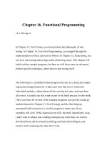
The book can be roughly divided into three parts, which are presented by different colors in Fig. 1.1.1:

Fig. 1.1.1: Book structure
• The first part covers prerequisites and basics. The first chapter offers an introduction to deep learning Section 3.

Then, in Section 4, we quickly bring you up to speed on the prerequisites required for hands-on deep learning, such
as how to store and manipulate data, and how to apply various numerical operations based on basic concepts from
linear algebra, calculus, and probability. Section 5 and Section 6 cover the most basic concepts and techniques of
deep learning, such as linear regression, multi-layer perceptrons and regularization.
• The next four chapters focus on modern deep learning techniques. Section 7 describes the various key components
of deep learning calculations and lays the groundwork for us to subsequently implement more complex models.
Next, in Section 8 and Section 9, we introduce Convolutional Neural Networks (CNNs), powerful tools that form
the backbone of most modern computer vision systems. Subsequently, in Section 10, we introduce Recurrent
Neural Networks (RNNS), models that exploit temporal or sequential structure in data, and are commonly used
for natural language processing and time series prediction. In Section 11, we introduce a new class of models that
employ a technique called an attention mechanism and that have recently begun to displace RNNs in NLP. These
sections will get you up to speed on the basic tools behind most modern applications of deep learning.
• Part three discusses scalability, efficiency and applications. First, in Section 12, we discuss several common optimization algorithms used to train deep learning models. The next chapter, Section 13 examines several key factors
that influence the computational performance of your deep learning code. In Section 14 and Section 15, we illus-

1.1. About This Book

3


Dive into Deep Learning, Release 0.7

trate major applications of deep learning in computer vision and natural language processing, respectively. Finally,
presents an emerging family of models called Generative Adversarial Networks (GANs).

1.1.4 Code
Most sections of this book feature executable code because of our belief in the importance of an interactive learning
experience in deep learning. At present, certain intuitions can only be developed through trial and error, tweaking the
code in small ways and observing the results. Ideally, an elegant mathematical theory might tell us precisely how to tweak
our code to achieve a desired result. Unfortunately, at present, such elegant theories elude us. Despite our best attempts,

formal explanations for various techniques are still lacking, both because the mathematics to charactize these models can
be so difficult and also because serious inquiry on these topics has only just recently kicked into high gear. We are hopeful
that as the theory of deep learning progresses, future editions of this book will be able to provide insights in places the
present edition cannot.
Most of the code in this book is based on Apache MXNet. MXNet is an open-source framework for deep learning and
the preferred choice of AWS (Amazon Web Services), as well as many colleges and companies. All of the code in this
book has passed tests under the newest MXNet version. However, due to the rapid development of deep learning, some
code in the print edition may not work properly in future versions of MXNet. However, we plan to keep the online version
remain up-to-date. In case you encounter any such problems, please consult Installation (page 7) to update your code and
runtime environment.
At times, to avoid unnecessary repetition, we encapsulate the frequently-imported and referred-to functions, classes, etc.
in this book in the d2l package. For any block block such as a function, a class, or multiple imports to be saved in
the package, we will mark it with # Saved in the d2l package for later use. The d2l package is
light-weight and only requires the following packages and modules as dependencies:
# Saved in the d2l package for later use
from IPython import display
import collections
from collections import defaultdict
import os
import sys
import math
from matplotlib import pyplot as plt
from mxnet import np, npx, autograd, gluon, init, context, image
from mxnet.gluon import nn, rnn
from mxnet.gluon.loss import Loss
from mxnet.gluon.data import Dataset
import random
import re
import time
import tarfile

import zipfile
import pandas as pd

We offer a detailed overview of these functions and classes in Section 19.5.

1.1.5 Target Audience
This book is for students (undergraduate or graduate), engineers, and researchers, who seek a solid grasp of the practical
techniques of deep learning. Because we explain every concept from scratch, no previous background in deep learning
or machine learning is required. Fully explaining the methods of deep learning requires some mathematics and programming, but we will only assume that you come in with some basics, including (the very basics of) linear algebra, calculus,
probability, and Python programming. Moreover, in the Appendix, we provide a refresher on most of the mathematics

4

Chapter 1. Preface


Dive into Deep Learning, Release 0.7

covered in this book. Most of the time, we will prioritize intuition and ideas over mathematical rigor. There are many
terrific books which can lead the interested reader further. For instance, Linear Analysis by Bela Bollobas (Bollobas,
1999) covers linear algebra and functional analysis in great depth. All of Statistics (Wasserman, 2013) is a terrific guide
to statistics. And if you have not used Python before, you may want to peruse this Python tutorial3 .

1.1.6 Forum
Associated with this book, we have launched a discussion forum, located at discuss.mxnet.io4 . When you have questions
on any section of the book, you can find the associated discussion page by scanning the QR code at the end of the section
to participate in its discussions. The authors of this book and broader MXNet developer community frequently participate
in forum discussions.

1.2 Acknowledgments

We are indebted to the hundreds of contributors for both the English and the Chinese drafts. They helped improve the
content and offered valuable feedback. Specifically, we thank every contributor of this English draft for making it better
for everyone. Their GitHub IDs or names are (in no particular order): alxnorden, avinashingit, bowen0701, brettkoonce,
Chaitanya Prakash Bapat, cryptonaut, Davide Fiocco, edgarroman, gkutiel, John Mitro, Liang Pu, Rahul Agarwal, Mohamed Ali Jamaoui, Michael (Stu) Stewart, Mike Müller, NRauschmayr, Prakhar Srivastav, sad-, sfermigier, Sheng
Zha, sundeepteki, topecongiro, tpdi, vermicelli, Vishaal Kapoor, vishwesh5, YaYaB, Yuhong Chen, Evgeniy Smirnov,
lgov, Simon Corston-Oliver, IgorDzreyev, Ha Nguyen, pmuens, alukovenko, senorcinco, vfdev-5, dsweet, Mohammad
Mahdi Rahimi, Abhishek Gupta, uwsd, DomKM, Lisa Oakley, Bowen Li, Aarush Ahuja, prasanth5reddy, brianhendee,
mani2106, mtn, lkevinzc, caojilin, Lakshya, Fiete Lüer, Surbhi Vijayvargeeya, Muhyun Kim, dennismalmgren, adursun,
Anirudh Dagar, liqingnz, Pedro Larroy, lgov, ati-ozgur, Jun Wu, Matthias Blume, Lin Yuan, geogunow, Josh Gardner,
Maximilian Böther, Rakib Islam, Leonard Lausen, Abhinav Upadhyay, rongruosong, Steve Sedlmeyer, ruslo, Rafael
Schlatter, liusy182, Giannis Pappas, ruslo, ati-ozgur, qbaza, dchoi77, Adam Gerson. Notably, Brent Werness (Amazon)
and Rachel Hu (Amazon) co-authored the Mathematics for Deep Learning chapter in the Appendix with us and are the
major contributors to that chapter.
We thank Amazon Web Services, especially Swami Sivasubramanian, Raju Gulabani, Charlie Bell, and Andrew Jassy
for their generous support in writing this book. Without the available time, resources, discussions with colleagues, and
continuous encouragement this book would not have happened.

1.3 Summary
• Deep learning has revolutionized pattern recognition, introducing technology that now powers a wide range of
technologies, including computer vision, natural language processing, automatic speech recognition.
• To successfully apply deep learning, you must understand how to cast a problem, the mathematics of modeling, the
algorithms for fitting your models to data, and the engineering techniques to implement it all.
• This book presents a comprehensive resource, including prose, figures, mathematics, and code, all in one place.
• To answer questions related to this book, visit our forum at />• Apache MXNet is a powerful library for coding up deep learning models and running them in parallel across GPU
cores.
• Gluon is a high level library that makes it easy to code up deep learning models using Apache MXNet.
• Conda is a Python package manager that ensures that all software dependencies are met.
3
4

/> />
1.2. Acknowledgments

5


Dive into Deep Learning, Release 0.7

• All notebooks are available for download on GitHub and the conda configurations needed to run this book’s code
are expressed in the environment.yml file.
• If you plan to run this code on GPUs, do not forget to install the necessary drivers and update your configuration.

1.4 Exercises
1. Register an account on the discussion forum of this book discuss.mxnet.io5 .
2. Install Python on your computer.
3. Follow the links at the bottom of the section to the forum, where you will be able to seek out help and discuss the
book and find answers to your questions by engaging the authors and broader community.
4. Create an account on the forum and introduce yourself.

1.5 Scan the QR Code to Discuss6

5
6

6

/> />
Chapter 1. Preface

CHAPTER

TWO

INSTALLATION

In order to get you up and running for hands-on learning experience, we need to set up you up with an environment for
running Python, Jupyter notebooks, the relevant libraries, and the code needed to run the book itself.

2.1 Installing Miniconda
The simplest way to get going will be to install Miniconda7 . Download the corresponding Miniconda “sh” file from the
website and then execute the installation from the command line using sudo sh <FILENAME> as follows:
# For Mac users (the file name is subject to changes)
sudo sh Miniconda3-latest-MacOSX-x86_64.sh
# For Linux users (the file name is subject to changes)
sudo sh Miniconda3-latest-Linux-x86_64.sh

You will be prompted to answer the following questions:
Do you accept the license terms? [yes|no]
[no] >>> yes
Miniconda3 will now be installed into this location:
/home/rlhu/miniconda3
- Press ENTER to confirm the location
- Press CTRL-C to abort the installation
- Or specify a different location below
>>> <ENTER>
Do you wish the installer to initialize Miniconda3
by running conda init? [yes|no]
[no] >>> yes

After installing miniconda, run the appropriate command (depending on your operating system) to activate conda.
# For Mac user
source ~/.bash_profile
# For Linux user
source ~/.bashrc

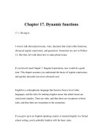
Then create the conda “d2l”” environment and enter y for the following inquiries as shown in Fig. 2.1.1.
7

/>
7


Dive into Deep Learning, Release 0.7

conda create --name d2l

Fig. 2.1.1: Conda create environment d2l.

2.2 Downloading the d2l Notebooks
Next, we need to download the code for this book.
sudo apt-get install unzip
mkdir d2l-en && cd d2l-en
wget />unzip d2l-en.zip && rm d2l-en.zip

Now we will now want to activate the “d2l” environment and install pip. Enter y for the queries that follow this command.
conda activate d2l
conda install python=3.7 pip

Finally, install the “d2l” package within the environment “d2l” that we created.

pip install git+ />
If everything went well up to now then you are almost there. If by some misfortune, something went wrong along the
way, please check the following:
1. That you are using pip for Python 3 instead of Python 2 by checking pip --version. If it is Python 2, then
you may check if there is a pip3 available.
2. That you are using a recent pip, such as version 19. If not, you can upgrade it via pip install --upgrade
pip.
3. Whether you have permission to install system-wide packages. If not, you can install to your home directory by
adding the flag --user to the pip command, e.g. pip install d2l --user.

2.3 Installing MXNet
Before installing mxnet, please first check whether or not you have proper GPUs on your machine (the GPUs that power
the display on a standard laptop do not count for our purposes. If you are installing on a GPU server, proceed to GPU
8

Chapter 2. Installation


Dive into Deep Learning, Release 0.7

Support (page 9) for instructions to install a GPU-supported mxnet.
Otherwise, you can install the CPU version. That will be more than enough horsepower to get you through the first few
chapters but you will want to access GPUs before running larger models.
# For Windows users
pip install mxnet==1.6.0b20190926
# For Linux and macOS users
pip install mxnet==1.6.0b20190915

Once both packages are installed, we now open the Jupyter notebook by running:
jupyter notebook

At this point, you can open http://localhost:8888 (it usually opens automatically) in your web browser. Once in the
notebook server, we can run the code for each section of the book.

2.4 Upgrade to a New Version
Both this book and MXNet are keeping improving. Please check a new version from time to time.
1. The URL always points to the latest contents.
2. Please upgrade “d2l” by pip install git+ />3. For the CPU version, MXNet can be upgraded by pip uninstall mxnet then re-running the aforementioned
pip install mxnet==... command.

2.5 GPU Support
By default, MXNet is installed without GPU support to ensure that it will run on any computer (including most laptops).
Part of this book requires or recommends running with GPU. If your computer has NVIDIA graphics cards and has
installed CUDA8 , then you should install a GPU-enabled MXNet. If you have installed the CPU-only version, you may
need to remove it first by running:
pip uninstall mxnet

Then we need to find the CUDA version you installed. You may check it through nvcc --version or cat /usr/
local/cuda/version.txt. Assume you have installed CUDA 10.1, then you can install the according MXNet
version with the following (OS-specific) command:
# For Windows users
pip install mxnet-cu101==1.6.0b20190926
# For Linux and macOS users
pip install mxnet-cu101==1.6.0b20190915

You may change the last digits according to your CUDA version, e.g., cu100 for CUDA 10.0 and cu90 for CUDA 9.0.
You can find all available MXNet versions via pip search mxnet.
For installation of MXNet on other platforms, please refer to />8

/>

2.4. Upgrade to a New Version

9


Dive into Deep Learning, Release 0.7

2.6 Exercises
1. Download the code for the book and install the runtime environment.

2.7 Scan the QR Code to Discuss9

9

10

/>
Chapter 2. Installation


CHAPTER

THREE

INTRODUCTION

Until recently, nearly every computer program that interact with daily were coded by software developers from first
principles. Say that we wanted to write an application to manage an e-commerce platform. After huddling around a
whiteboard for a few hours to ponder the problem, we would come up with the broad strokes of a working solution that
might probably look something like this: (i) users interact with the application through an interface running in a web

browser or mobile application; (ii) our application interacts with a commercial-grade database engine to keep track of
each user’s state and maintain records of historical transactions; and (iii) at the heart of our application, the business logic
(you might say, the brains) of our application spells out in methodical detail the appropriate action that our program should
take in every conceivable circumstance.
To build the brains of our application, we’d have to step through every possible corner case that we anticipate encountering,
devising appropriate rules. Each time a customer clicks to add an item to their shopping cart, we add an entry to the
shopping cart database table, associating that user’s ID with the requested product’s ID. While few developers ever get it
completely right the first time (it might take some test runs to work out the kinks), for the most part, we could write such a
program from first principles and confidently launch it before ever seeing a real customer. Our ability to design automated
systems from first principles that drive functioning products and systems, often in novel situations, is a remarkable cognitive
feat. And when you are able to devise solutions that work 100% of the time, you should not be using machine learning.
Fortunately for the growing community of ML scientists, many tasks that we would like to automate do not bend so easily
to human ingenuity. Imagine huddling around the whiteboard with the smartest minds you know, but this time you are
tackling one of the following problems:
• Write a program that predicts tomorrow’s weather given geographic information, satellite images, and a trailing
window of past weather.
• Write a program that takes in a question, expressed in free-form text, and answers it correctly.
• Write a program that given an image can identify all the people it contains, drawing outlines around each.
• Write a program that presents users with products that they are likely to enjoy but unlikely, in the natural course of
browsing, to encounter.
In each of these cases, even elite programmers are incapable of coding up solutions from scratch. The reasons for this
can vary. Sometimes the program that we are looking for follows a pattern that changes over time, and we need our
programs to adapt. In other cases, the relationship (say between pixels, and abstract categories) may be too complicated,
requiring thousands or millions of computations that are beyond our conscious understanding (even if our eyes manage
the task effortlessly). Machine learning (ML) is the study of powerful techniques that can learn from experience. As ML
algorithm accumulates more experience, typically in the form of observational data or interactions with an environment,
their performance improves. Contrast this with our deterministic e-commerce platform, which performs according to the
same business logic, no matter how much experience accrues, until the developers themselves learn and decide that it is
time to update the software. In this book, we will teach you the fundamentals of machine learning, and focus in particular
on deep learning, a powerful set of techniques driving innovations in areas as diverse as computer vision, natural language

processing, healthcare, and genomics.

11


Dive into Deep Learning, Release 0.7

3.1 A Motivating Example
Before we could begin writing, the authors of this book, like much of the work force, had to become caffeinated. We
hopped in the car and started driving. Using an iPhone, Alex called out ‘Hey Siri’, awakening the phone’s voice recognition
system. Then Mu commanded ‘directions to Blue Bottle coffee shop’. The phone quickly displayed the transcription of his
command. It also recognized that we were asking for directions and launched the Maps application to fulfill our request.
Once launched, the Maps app identified a number of routes. Next to each route, the phone displayed a predicted transit
time. While we fabricated this story for pedagogical convenience, it demonstrates that in the span of just a few seconds,
our everyday interactions with a smart phone can engage several machine learning models.
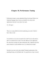
Imagine just writing a program to respond to a wake word like ‘Alexa’, ‘Okay, Google’ or ‘Siri’. Try coding it up in a room
by yourself with nothing but a computer and a code editor. How would you write such a program from first principles?
Think about it… the problem is hard. Every second, the microphone will collect roughly 44,000 samples. Each sample is
a measurement of the amplitude of the sound wave. What rule could map reliably from a snippet of raw audio to confident
predictions {yes, no} on whether the snippet contains the wake word? If you are stuck, do not worry. We do not
know how to write such a program from scratch either. That is why we use ML.

Fig. 3.1.1: Identify an awake word.
Here’s the trick. Often, even when we do not know how to tell a computer explicitly how to map from inputs to outputs,
we are nonetheless capable of performing the cognitive feat ourselves. In other words, even if you do not know how to
program a computer to recognize the word ‘Alexa’, you yourself are able to recognize the word ‘Alexa’. Armed with this
ability, we can collect a huge dataset containing examples of audio and label those that do and that do not contain the
wake word. In the ML approach, we do not attempt to design a system explicitly to recognize wake words. Instead, we
define a flexible program whose behavior is determined by a number of parameters. Then we use the dataset to determine
the best possible set of parameters, those that improve the performance of our program with respect to some measure of

performance on the task of interest.
You can think of the parameters as knobs that we can turn, manipulating the behavior of the program. Fixing the
parameters, we call the program a model. The set of all distinct programs (input-output mappings) that we can produce
just by manipulating the parameters is called a family of models. And the meta-program that uses our dataset to choose
the parameters is called a learning algorithm.
Before we can go ahead and engage the learning algorithm, we have to define the problem precisely, pinning down the
exact nature of the inputs and outputs, and choosing an appropriate model family. In this case, our model receives a
snippet of audio as input, and it generates a selection among {yes, no} as output. If all goes according to plan the
model’s guesses will typically be correct as to whether (or not) the snippet contains the wake word.

If we choose the right family of models, then there should exist one setting of the knobs such that the model fires yes
every time it hears the word ‘Alexa’. Because the exact choice of the wake word is arbitrary, we will probably need a
model family sufficiently rich that, via another setting of the knobs, it could fire yes only upon hearing the word
‘Apricot’. We expect that the same model family should be suitable for ‘Alexa’ recognition and ‘Apricot’ recognition
because they seem, intuitively, to be similar tasks.
However, we might need a different family of models entirely if we want to deal with fundamentally different inputs or
outputs, say if we wanted to map from images to captions, or from English sentences to Chinese sentences.

As you might guess, if we just set all of the knobs randomly, it is not likely that our model will recognize ‘Alexa’, ‘Apricot’,
or any other English word. In deep learning, the learning is the process by which we discover the right setting of the knobs
12

Chapter 3. Introduction


Dive into Deep Learning, Release 0.7

coercing the desired behavior from our model.
The training process usually looks like this:
1. Start off with a randomly initialized model that cannot do anything useful.

2. Grab some of your labeled data (e.g., audio snippets and corresponding {yes,no} labels)
3. Tweak the knobs so the model sucks less with respect to those examples
4. Repeat until the model is awesome.

Fig. 3.1.2: A typical training process.
To summarize, rather than code up a wake word recognizer, we code up a program that can learn to recognize wake words,
if we present it with a large labeled dataset. You can think of this act of determining a program’s behavior by presenting
it with a dataset as programming with data. We can “program” a cat detector by providing our machine learning system
with many examples of cats and dogs, such as the images below:

cat

cat

dog

dog

This way the detector will eventually learn to emit a very large positive number if it is a cat, a very large negative number
if it is a dog, and something closer to zero if it is not sure, and this barely scratches the surface of what ML can do.
Deep learning is just one among many popular methods for solving machine learning problems. Thus far, we have only
talked about machine learning broadly and not deep learning. To see why deep learning is important, we should pause
for a moment to highlight a couple crucial points.
First, the problems that we have discussed thus far—learning from raw audio signal, the raw pixel values of images, or
mapping between sentences of arbitrary lengths and their counterparts in foreign languages—are problems where deep
learning excels and where traditional ML methods faltered. Deep models are deep in precisely the sense that they learn
many layers of computation. It turns out that these many-layered (or hierarchical) models are capable of addressing lowlevel perceptual data in a way that previous tools could not. In bygone days, the crucial part of applying ML to these
problems consisted of coming up with manually-engineered ways of transforming the data into some form amenable to
shallow models. One key advantage of deep learning is that it replaces not only the shallow models at the end of traditional

3.1. A Motivating Example

13


Dive into Deep Learning, Release 0.7

learning pipelines, but also the labor-intensive process of feature engineering. Secondly, by replacing much of the domainspecific preprocessing, deep learning has eliminated many of the boundaries that previously separated computer vision,
speech recognition, natural language processing, medical informatics, and other application areas, offering a unified set
of tools for tackling diverse problems.

3.2 The Key Components: Data, Models, and Algorithms
In our wake-word example, we described a dataset consisting of audio snippets and binary labels gave a hand-wavy sense
of how we might train a model to approximate a mapping from snippets to classifications. This sort of problem, where
we try to predict a designated unknown label given known inputs, given a dataset consisting of examples, for which the
labels are known is called supervised learning, and it is just one among many kinds of machine learning problems. In the
next section, we will take a deep dive into the different ML problems. First, we’d like to shed more light on some core
components that will follow us around, no matter what kind of ML problem we take on:
1. The data that we can learn from.
2. A model of how to transform the data.
3. A loss function that quantifies the badness of our model.
4. An algorithm to adjust the model’s parameters to minimize the loss.

3.2.1 Data
It might go without saying that you cannot do data science without data. We could lose hundreds of pages pondering what
precisely constitutes data, but for now we will err on the practical side and focus on the key properties to be concerned
with. Generally we are concerned with a collection of examples (also called data points, samples, or instances). In order
to work with data usefully, we typically need to come up with a suitable numerical representation. Each example typically
consists of a collection of numerical attributes called features. In the supervised learning problems above, a special feature
is designated as the prediction target, (sometimes called the label or dependent variable). The given features from which

the model must make its predictions can then simply be called the features, (or often, the inputs, covariates, or independent
variables).
If we were working with image data, each individual photograph might constitute an example, each represented by an
ordered list of numerical values corresponding to the brightness of each pixel. A 200 × 200 color photograph would
consist of 200 × 200 × 3 = 120000 numerical values, corresponding to the brightness of the red, green, and blue
channels for each spatial location. In a more traditional task, we might try to predict whether or not a patient will survive,
given a standard set of features such as age, vital signs, diagnoses, etc.
When every example is characterized by the same number of numerical values, we say that the data consists of fixed-length
vectors and we describe the (constant) length of the vectors as the dimensionality of the data. As you might imagine, fixed
length can be a convenient property. If we wanted to train a model to recognize cancer in microscopy images, fixed-length
inputs means we have one less thing to worry about.
However, not all data can easily be represented as fixed length vectors. While we might expect microscrope images to
come from standard equipment, we cannot expect images mined from the Internet to all show up with the same resolution
or shape. For images, we might consider cropping them all to a standard size, but that strategy only gets us so far. We
risk losing information in the cropped out portions. Moreover, text data resists fixed-length representations even more
stubbornly. Consider the customer reviews left on e-commerce sites like Amazon, IMDB, or TripAdvisor. Some are short:
“it stinks!”. Others ramble for pages. One major advantage of deep learning over traditional methods is the comparative
grace with which modern models can handle varying-length data.
Generally, the more data we have, the easier our job becomes. When we have more data, we can train more powerful
models, and rely less heavily on pre-conceived assumptions. The regime change from (comparatively small) to big data is
a major contributor to the success of modern deep learning. To drive the point home, many of the most exciting models

14

Chapter 3. Introduction


Dive into Deep Learning, Release 0.7

in deep learning either do not work without large datasets. Some others work in the low-data regime, but no better than

traditional approaches.
Finally it is not enough to have lots of data and to process it cleverly. We need the right data. If the data is full of
mistakes, or if the chosen features are not predictive of the target quantity of interest, learning is going to fail. The
situation is captured well by the cliché: garbage in, garbage out. Moreover, poor predictive performance is not the only
potential consequence. In sensitive applications of machine learning, like predictive policing, resumé screening, and risk
models used for lending, we must be especially alert to the consequences of garbage data. One common failure mode
occurs in datasets where some groups of people are unrepresented in the training data. Imagine applying a skin cancer
recognition system in the wild that had never seen black skin before. Failure can also occur when the data does not
merely under-represent some groups, but reflects societal prejudices. For example if past hiring decisions are used to
train a predictive model that will be used to screen resumes, then machine learning models could inadvertently capture
and automate historical injustices. Note that this can all happen without the data scientist actively conspiring, or even
being aware.

3.2.2 Models
Most machine learning involves transforming the data in some sense. We might want to build a system that ingests
photos and predicts smiley-ness. Alternatively, we might want to ingest a set of sensor readings and predict how normal vs
anomalous the readings are. By model, we denote the computational machinery for ingesting data of one type, and spitting
out predictions of a possibly different type. In particular, we are interested in statistical models that can be estimated from
data. While simple models are perfectly capable of addressing appropriately simple problems the problems that we focus
on in this book stretch the limits of classical methods. Deep learning is differentiated from classical approaches principally
by the set of powerful models that it focuses on. These models consist of many successive transformations of the data that
are chained together top to bottom, thus the name deep learning. On our way to discussing deep neural networks, we will
discuss some more traditional methods.

3.2.3 Objective functions
Earlier, we introduced machine learning as “learning from experience”. By learning here, we mean improving at some
task over time. But who is to say what constitutes an improvement? You might imagine that we could propose to update
our model, and some people might disagree on whether the proposed update constituted an improvement or a decline.
In order to develop a formal mathematical system of learning machines, we need to have formal measures of how good
(or bad) our models are. In machine learning, and optimization more generally, we call these objective functions. By

convention, we usually define objective functions so that lower is better. This is merely a convention. You can take any
function f for which higher is better, and turn it into a new function f ′ that is qualitatively identical but for which lower is
better by setting f ′ = −f . Because lower is better, these functions are sometimes called loss functions or cost functions.
When trying to predict numerical values, the most common objective function is squared error (y − yˆ)2 . For classification,
the most common objective is to minimize error rate, i.e., the fraction of instances on which our predictions disagree
with the ground truth. Some objectives (like squared error) are easy to optimize. Others (like error rate) are difficult
to optimize directly, owing to non-differentiability or other complications. In these cases, it is common to optimize a
surrogate objective.
Typically, the loss function is defined with respect to the model’s parameters and depends upon the dataset. The best
values of our model’s parameters are learned by minimizing the loss incurred on a training set consisting of some number
of examples collected for training. However, doing well on the training data does not guarantee that we will do well on
(unseen) test data. So we will typically want to split the available data into two partitions: the training data (for fitting
model parameters) and the test data (which is held out for evaluation), reporting the following two quantities:
• Training Error: The error on that data on which the model was trained. You could think of this as being like a
student’s scores on practice exams used to prepare for some real exam. Even if the results are encouraging, that
does not guarantee success on the final exam.

3.2. The Key Components: Data, Models, and Algorithms

15


Dive into Deep Learning, Release 0.7

• Test Error: This is the error incurred on an unseen test set. This can deviate significantly from the training error.
When a model performs well on the training data but fails to generalize to unseen data, we say that it is overfitting.
In real-life terms, this is like flunking the real exam despite doing well on practice exams.

3.2.4 Optimization algorithms
Once we have got some data source and representation, a model, and a well-defined objective function, we need an

algorithm capable of searching for the best possible parameters for minimizing the loss function. The most popular
optimization algorithms for neural networks follow an approach called gradient descent. In short, at each step, they check
to see, for each parameter, which way the training set loss would move if you perturbed that parameter just a small
amount. They then update the parameter in the direction that reduces the loss.

3.3 Kinds of Machine Learning
In the following sections, we discuss a few kinds of machine learning problems in greater detail. We begin with a list of
objectives, i.e., a list of things that we would like machine learning to do. Note that the objectives are complemented with
a set of techniques of how to accomplish them, including types of data, models, training techniques, etc. The list below
is just a sampling of the problems ML can tackle to motivate the reader and provide us with some common language for
when we talk about more problems throughout the book.

3.3.1 Supervised learning
Supervised learning addresses the task of predicting targets given inputs. The targets, which we often call labels, are
generally denoted by y. The input data, also called the features or covariates, are typically denoted x. Each (input, target)
pair is called an examples or an instances. Some times, when the context is clear, we may use the term examples, to refer
to a collection of inputs, even when the corresponding targets are unknown. We denote any particular instance with a
subscript, typicaly i, for instance (xi , y_i). A dataset is a collection of n instances {xi , yi }ni=1 . Our goal is to produce a
model fθ that maps any input xi to a prediction fθ (xi )
To ground this description in a concrete example, if we were working in healthcare, then we might want to predict whether
or not a patient would have a heart attack. This observation, heart attack or no heart attack, would be our label y. The
input data x might be vital signs such as heart rate, diastolic and systolic blood pressure, etc.
The supervision comes into play because for choosing the parameters θ, we (the supervisors) provide the model with a
dataset consisting of labeled examples (xi , yi ), where each example xi is matched with the correct label.
In probabilistic terms, we typically are interested in estimating the conditional probability P (y|x). While it is just one
among several paradigms within machine learning, supervised learning accounts for the majority of successful applications
of machine learning in industry. Partly, that is because many important tasks can be described crisply as estimating the
probability of something unknown given a particular set of available data:
• Predict cancer vs not cancer, given a CT image.
• Predict the correct translation in French, given a sentence in English.

• Predict the price of a stock next month based on this month’s financial reporting data.
Even with the simple description “predict targets from inputs” supervised learning can take a great many forms and require
a great many modeling decisions, depending on (among other considerations) the type, size, and the number of inputs
and outputs. For example, we use different models to process sequences (like strings of text or time series data) and for
processing fixed-length vector representations. We will visit many of these problems in depth throughout the first 9 parts
of this book.

16

Chapter 3. Introduction


Dive into Deep Learning, Release 0.7

Informally, the learning process looks something like this: Grab a big collection of examples for which the covariates are
known and select from them a random subset, acquiring the ground truth labels for each. Sometimes these labels might
be available data that has already been collected (e.g., did a patient die within the following year?) and other times we
might need to employ human annotators to label the data, (e.g., assigning images to categories).
Together, these inputs and corresponding labels comprise the training set. We feed the training dataset into a supervised
learning algorithm, a function that takes as input a dataset and outputs another function, the learned model. Finally, we
can feed previously unseen inputs to the learned model, using its outputs as predictions of the corresponding label.

Fig. 3.3.1: Supervised learning.

Regression
Perhaps the simplest supervised learning task to wrap your head around is regression. Consider, for example a set of data
harvested from a database of home sales. We might construct a table, where each row corresponds to a different house,
and each column corresponds to some relevant attribute, such as the square footage of a house, the number of bedrooms,
the number of bathrooms, and the number of minutes (walking) to the center of town. In this dataset each example would
be a specific house, and the corresponding feature vector would be one row in the table.

If you live in New York or San Francisco, and you are not the CEO of Amazon, Google, Microsoft, or Facebook, the (sq.
footage, no. of bedrooms, no. of bathrooms, walking distance) feature vector for your home might look something like:
[100, 0, .5, 60]. However, if you live in Pittsburgh, it might look more like [3000, 4, 3, 10]. Feature vectors like this are
essential for most classic machine learning algorithms. We will continue to denote the feature vector correspond to any
example i as xi and we can compactly refer to the full table containing all of the feature vectors as X.
What makes a problem a regression is actually the outputs. Say that you are in the market for a new home. You might
want to estimate the fair market value of a house, given some features like these. The target value, the price of sale,
is a real number. If you remember the formal definition of the reals you might be scratching your head now. Homes
probably never sell for fractions of a cent, let alone prices expressed as irrational numbers. In cases like this, when the
target is actually discrete, but where the rounding takes place on a sufficiently fine scale, we will abuse language just a bit
cn continue to describe our outputs and targets as real-valued numbers.
We denote any individual target yi (corresponding to example xi ) and the set of all targets y (corresponding to all examples
X). When our targets take on arbitrary values in some range, we call this a regression problem. Our goal is to produce
a model whose predictions closely approximate the actual target values. We denote the predicted target for any instance
yˆi . Do not worry if the notation is bogging you down. We will unpack it more thoroughly in the subsequent chapters.
Lots of practical problems are well-described regression problems. Predicting the rating that a user will assign to a movie
can be thought of as a regression problem and if you designed a great algorithm to accomplish this feat in 2009, you
might have won the $1 million Netflix prize10 . Predicting the length of stay for patients in the hospital is also a regression
problem. A good rule of thumb is that any How much? or How many? problem should suggest regression.
• ‘How many hours will this surgery take?’ - regression
• ‘How many dogs are in this photo?’ - regression.
10

/>
3.3. Kinds of Machine Learning

17


Dive into Deep Learning, Release 0.7

However, if you can easily pose your problem as ‘Is this a _ ?’, then it is likely, classification, a different kind of supervised
problem that we will cover next. Even if you have never worked with machine learning before, you have probably worked
through a regression problem informally. Imagine, for example, that you had your drains repaired and that your contractor
spent x1 = 3 hours removing gunk from your sewage pipes. Then she sent you a bill of y1 = $350. Now imagine that
your friend hired the same contractor for x2 = 2 hours and that she received a bill of y2 = $250. If someone then asked
you how much to expect on their upcoming gunk-removal invoice you might make some reasonable assumptions, such
as more hours worked costs more dollars. You might also assume that there is some base charge and that the contractor
then charges per hour. If these assumptions held true, then given these two data points, you could already identify the
contractor’s pricing structure: $100 per hour plus $50 to show up at your house. If you followed that much then you
already understand the high-level idea behind linear regression (and you just implicitly designed a linear model with a bias
term).
In this case, we could produce the parameters that exactly matched the contractor’s prices. Sometimes that is not possible,
e.g., if some of the variance owes to some factors besides your two features. In these cases, we will try to learn models
that minimize the distance between our predictions and the observed values. In most of our chapters, we will focus on
one of two very common losses, the L1 loss11 where
∑
l(y, y ′ ) =
|yi − yi′ |
(3.3.1)
i

and the least mean squares loss, or L2 loss12 , where
l(y, y ′ ) =

∑
(yi − yi′ )2 .

(3.3.2)

i

As we will see later, the L2 loss corresponds to the assumption that our data was corrupted by Gaussian noise, whereas
the L1 loss corresponds to an assumption of noise from a Laplace distribution.
Classification
While regression models are great for addressing how many? questions, lots of problems do not bend comfortably to this
template. For example, a bank wants to add check scanning to their mobile app. This would involve the customer snapping
a photo of a check with their smart phone’s camera and the machine learning model would need to be able to automatically
understand text seen in the image. It would also need to understand hand-written text to be even more robust. This kind of
system is referred to as optical character recognition (OCR), and the kind of problem it addresses is called classification.
It is treated with a different set of algorithms than those used for regression (although many techniques will carry over).
In classification, we want our model to look at a feature vector, e.g. the pixel values in an image, and then predict which
category (formally called classes), among some (discrete) set of options, an example belongs. For hand-written digits, we
might have 10 classes, corresponding to the digits 0 through 9. The simplest form of classification is when there are only
two classes, a problem which we call binary classification. For example, our dataset X could consist of images of animals
and our labels Y might be the classes {cat, dog}. While in regression, we sought a regressor to output a real value yˆ, in
classification, we seek a classifier, whose output yˆ is the predicted class assignment.
For reasons that we will get into as the book gets more technical, it can be hard to optimize a model that can only output
a hard categorical assignment, e.g., either cat or dog. In these cases, it is usually much easier to instead express our model
in the language of probabilities. Given an example x, our model assigns a probability yˆk to each label k. Because these
are probabilities, they need to be positive numbers and add up to 1 and thus we only need K − 1 numbers to assign
probabilities of K categories. This is easy to see for binary classification. If there is a 0.6 (60%) probability that an unfair
coin comes up heads, then there is a 0.4 (40%) probability that it comes up tails. Returning to our animal classification
example, a classifier might see an image and output the probability that the image is a cat P (y = cat|x) = 0.9. We
can interpret this number by saying that the classifier is 90% sure that the image depicts a cat. The magnitude of the
probability for the predicted class conveys one notion of uncertainty. It is not the only notion of uncertainty and we will
discuss others in more advanced chapters.
11
12

18

/> />
Chapter 3. Introduction


Dive into Deep Learning, Release 0.7

When we have more than two possible classes, we call the problem multiclass classification. Common examples include
hand-written character recognition [0, 1, 2, 3 ... 9, a, b, c, ...]. While we attacked regression problems by trying to minimize the L1 or L2 loss functions, the common loss function for classification problems is called
cross-entropy. In MXNet Gluon, the corresponding loss function can be found here13 .
Note that the most likely class is not necessarily the one that you are going to use for your decision. Assume that you find
this beautiful mushroom in your backyard:

Fig. 3.3.2: Death cap - do not eat!
Now, assume that you built a classifier and trained it to predict if a mushroom is poisonous based on a photograph. Say
our poison-detection classifier outputs P (y = deathcap|image) = 0.2. In other words, the classifier is 80% sure that our
mushroom is not a death cap. Still, you’d have to be a fool to eat it. That is because the certain benefit of a delicious
dinner is not worth a 20% risk of dying from it. In other words, the effect of the uncertain risk outweighs the benefit by
far. We can look at this more formally. Basically, we need to compute the expected risk that we incur, i.e., we need to
multiply the probability of the outcome with the benefit (or harm) associated with it:
L(action|x) = Ey∼p(y|x) [loss(action, y)]

(3.3.3)

Hence, the loss L incurred by eating the mushroom is L(a = eat|x) = 0.2 ∗ ∞ + 0.8 ∗ 0 = ∞, whereas the cost of
discarding it is L(a = discard|x) = 0.2 ∗ 0 + 0.8 ∗ 1 = 0.8.
Our caution was justified: as any mycologist would tell us, the above mushroom actually is a death cap. Classification
can get much more complicated than just binary, multiclass, or even multi-label classification. For instance, there are
some variants of classification for addressing hierarchies. Hierarchies assume that there exist some relationships among

13

/>
3.3. Kinds of Machine Learning

19