Báo cáo khoa học: "A Cascaded Linear Model for Joint Chinese Word Segmentation and Part-of-Speech Tagging" pdf
Bạn đang xem bản rút gọn của tài liệu. Xem và tải ngay bản đầy đủ của tài liệu tại đây (197.81 KB, 8 trang )
Proceedings of ACL-08: HLT, pages 897–904,
Columbus, Ohio, USA, June 2008.
c
2008 Association for Computational Linguistics
A Cascaded Linear Model for Joint Chinese Word Segmentation and
Part-of-Speech Tagging
Wenbin Jiang
†
Liang Huang
‡
Qun Liu
†
Yajuan L
¨
u
†
†
Key Lab. of Intelligent Information Processing
‡
Department of Computer & Information Science
Institute of Computing Technology University of Pennsylvania
Chinese Academy of Sciences Levine Hall, 3330 Walnut Street
P.O. Box 2704, Beijing 100190, China Philadelphia, PA 19104, USA
Abstract
We propose a cascaded linear model for
joint Chinese word segmentation and part-
of-speech tagging. With a character-based
perceptron as the core, combined with real-
valued features such as language models, the
cascaded model is able to efficiently uti-
lize knowledge sources that are inconvenient
to incorporate into the perceptron directly.
Experiments show that the cascaded model
achieves improved accuracies on both seg-
mentation only and joint segmentation and
part-of-speech tagging. On the Penn Chinese
Treebank 5.0, we obtain an error reduction of
18.5% on segmentation and 12% on joint seg-
mentation and part-of-speech tagging over the
perceptron-only baseline.
1 Introduction
Word segmentation and part-of-speech (POS) tag-
ging are important tasks in computer processing of
Chinese and other Asian languages. Several mod-
els were introduced for these problems, for example,
the Hidden Markov Model (HMM) (Rabiner, 1989),
Maximum Entropy Model (ME) (Ratnaparkhi and
Adwait, 1996), and Conditional Random Fields
(CRFs) (Lafferty et al., 2001). CRFs have the ad-
vantage of flexibility in representing features com-
pared to generative ones such as HMM, and usually
behaves the best in the two tasks. Another widely
used discriminative method is the perceptron algo-
rithm (Collins, 2002), which achieves comparable
performance to CRFs with much faster training, so
we base this work on the perceptron.
To segment and tag a character sequence, there
are two strategies to choose: performing POS tag-
ging following segmentation; or joint segmentation
and POS tagging (Joint S&T). Since the typical ap-
proach of discriminative models treats segmentation
as a labelling problem by assigning each character
a boundary tag (Xue and Shen, 2003), Joint S&T
can be conducted in a labelling fashion by expand-
ing boundary tags to include POS information (Ng
and Low, 2004). Compared to performing segmen-
tation and POS tagging one at a time, Joint S&T can
achieve higher accuracy not only on segmentation
but also on POS tagging (Ng and Low, 2004). Be-
sides the usual character-based features, additional
features dependent on POS’s or words can also be
employed to improve the performance. However, as
such features are generated dynamically during the
decoding procedure, two limitation arise: on the one
hand, the amount of parameters increases rapidly,
which is apt to overfit on training corpus; on the
other hand, exact inference by dynamic program-
ming is intractable because the current predication
relies on the results ofprior predications. As a result,
many theoretically useful features such as higher-
order word or POS n-grams are difficult to be in-
corporated in the model efficiently.
To cope with this problem, we propose a cascaded
linear model inspired by the log-linear model (Och
and Ney, 2004) widely used in statistical machine
translation to incorporate different kinds of knowl-
edge sources. Shown in Figure 1, the cascaded
model has a two-layer architecture, with a character-
based perceptron as the core combined with other
real-valued features such as language models. We
897
Core
Linear Model
(Perceptron)
g
1
=
i
α
i
× f
i
α
Outside-layer
Linear Model
S =
j
w
j
× g
j
w
f
1
f
2
f
|R|
g
1
Word LM: g
2
= P
wlm
(W )
g
2
POS LM: g
3
= P
tlm
(T )
g
3
Labelling: g
4
= P (T |W )
g
4
Generating: g
5
= P (W |T )
g
5
Length: g
6
= |W |
g
6
S
Figure 1: Structure of Cascaded Linear Model. |R| denotes the scale of the feature space of the core perceptron.
will describe it in detail in Section 4. In this ar-
chitecture, knowledge sources that are intractable to
incorporate into the perceptron, can be easily incor-
porated into the outside linear model. In addition,
as these knowledge sources are regarded as separate
features, we can train their corresponding models in-
dependently with each other. This is an interesting
approach when the training corpus is large as it re-
duces the time and space consumption. Experiments
show that our cascaded model can utilize different
knowledge sources effectively and obtain accuracy
improvements on both segmentation and Joint S&T.
2 Segmentation and POS Tagging
Given a Chinese character sequence:
C
1:n
= C
1
C
2
C
n
the segmentation result can be depicted as:
C
1:e
1
C
e
1
+1:e
2
C
e
m−1
+1:e
m
while the segmentation and POS tagging result can
be depicted as:
C
1:e
1
/t
1
C
e
1
+1:e
2
/t
2
C
e
m−1
+1:e
m
/t
m
Here, C
i
(i = 1 n) denotes Chinese character,
t
i
(i = 1 m) denotes POS tag, and C
l:r
(l ≤ r)
denotes character sequence ranges from C
l
to C
r
.
We can see that segmentation and POS tagging task
is to divide a character sequence into several subse-
quences and label each of them a POS tag.
It is a better idea to perform segmentation and
POS tagging jointly in a uniform framework. Ac-
cording to Ng and Low (2004), the segmentation
task can be transformed to a tagging problem by as-
signing each character a boundary tag of the follow-
ing four types:
• b: the begin of the word
• m: the middle of the word
• e: the end of the word
• s: a single-character word
We can extract segmentation result by splitting
the labelled result into subsequences of pattern s or
bm
∗
e which denote single-character word and multi-
character word respectively. In order to perform
POS tagging at the same time, we expand boundary
tags to include POS information by attaching a POS
to the tail of a boundary tag as a postfix following
Ng and Low (2004). As each tag is now composed
of a boundary part and a POS part, the joint S&T
problem is transformed to a uniform boundary-POS
labelling problem. A subsequence of boundary-POS
labelling result indicates a word with POS t only if
the boundary tag sequence composed of its bound-
ary part conforms to s or bm
∗
e style, and all POS
tags in its POS part equal to t. For example, a tag
sequence b
NN m NN e NN represents a three-
character word with POS tag NN.
3 The Perceptron
The perceptron algorithm introduced into NLP by
Collins (2002), is a simple but effective discrimina-
tive training method. It has comparable performance
898
Non-lexical-target Instances
C
n
(n = −2 2) C
−2
=, C
−1
=, C
0
=, C
1
=, C
2
=
C
n
C
n+1
(n = −2 1) C
−2
C
−1
=, C
−1
C
0
=, C
0
C
1
=, C
1
C
2
=
C
−1
C
1
C
−1
C
1
=
Lexical-target Instances
C
0
C
n
(n = −2 2) C
0
C
−2
=, C
0
C
−1
=, C
0
C
0
=, C
0
C
1
=, C
0
C
2
=
C
0
C
n
C
n+1
(n = −2 1) C
0
C
−2
C
−1
=, C
0
C
−1
C
0
=, C
0
C
0
C
1
=, C
0
C
1
C
2
=
C
0
C
−1
C
1
C
0
C
−1
C
1
=
Table 1: Feature templates and instances. Suppose we are considering the third character ”” in ” ”.
to CRFs, while with much faster training. The per-
ceptron has been used in many NLP tasks, such as
POS tagging (Collins, 2002), Chinese word seg-
mentation (Ng and Low, 2004; Zhang and Clark,
2007) and so on. We trained a character-based per-
ceptron for Chinese Joint S&T, and found that the
perceptron itself could achieve considerably high ac-
curacy on segmentation and Joint S&T. In following
subsections, we describe the feature templates and
the perceptron training algorithm.
3.1 Feature Templates
The feature templates we adopted are selected from
those of Ng and Low (2004). To compare with oth-
ers conveniently, we excluded the ones forbidden by
the close test regulation of SIGHAN, for example,
P u(C
0
), indicating whether character C
0
is a punc-
tuation.
All feature templates and their instances are
shown in Table 1. C represents a Chinese char-
acter while the subscript of C indicates its posi-
tion in the sentence relative to the current charac-
ter (it has the subscript 0). Templates immediately
borrowed from Ng and Low (2004) are listed in
the upper column named non-lexical-target. We
called them non-lexical-target because predications
derived from them can predicate without consider-
ing the current character C
0
. Templates in the col-
umn below are expanded from the upper ones. We
add a field C
0
to each template in the upper col-
umn, so that it can carry out predication according
to not only the context but also the current char-
acter itself. As predications generated from such
templates depend on the current character, we name
these templates lexical-target. Note that the tem-
plates of Ng and Low (2004) have already con-
tained some lexical-target ones. With the two kinds
Algorithm 1 Perceptron training algorithm.
1: Input: Training examples (x
i
, y
i
)
2: α ← 0
3: for t ← 1 T do
4: for i ← 1 N do
5: z
i
← argmax
z∈GEN(x
i
)
Φ(x
i
, z) · α
6: if z
i
= y
i
then
7: α ← α + Φ(x
i
, y
i
) − Φ(x
i
, z
i
)
8: Output: Parameters α
of predications, the perceptron model will do exact
predicating to the best of its ability, and can back
off to approximately predicating if exact predicating
fails.
3.2 Training Algorithm
We adopt the perceptron training algorithm of
Collins (2002) to learn a discriminative model map-
ping from inputs x ∈ X to outputs y ∈ Y , where X
is the set of sentences in the training corpus and Y
is the set of corresponding labelled results. Follow-
ing Collins, we use a function GEN(x) generating
all candidate results of an input x , a representation
Φ mapping each training example (x, y) ∈ X × Y
to a feature vector Φ(x, y) ∈ R
d
, and a parameter
vector α ∈ R
d
corresponding to the feature vector.
d means the dimension of the vector space, it equals
to the amount of features in the model. For an input
character sequence x, we aim to find an output F(x)
satisfying:
F (x) = argmax
y∈GEN(x)
Φ(x, y) · α (1)
Φ(x, y) · α represents the inner product of feature
vector Φ(x, y) and the parameter vector α. We used
the algorithm depicted in Algorithm 1 to tune the
parameter vector α.
899
To alleviate overfitting on the training examples,
we use the refinement strategy called “averaged pa-
rameters” (Collins, 2002) to the algorithm in Algo-
rithm 1.
4 Cascaded Linear Model
In theory, any useful knowledge can be incorporated
into the perceptron directly, besides the character-
based features already adopted. Additional features
most widely used are related to word or POS n-
grams. However, such features are generated dy-
namically during the decoding procedure so that
the feature space enlarges much more rapidly. Fig-
ure 2 shows the growing tendency of feature space
with the introduction of these features as well as the
character-based ones. We noticed that the templates
related to word unigrams and bigrams bring to the
feature space an enlargement much rapider than the
character-base ones, not to mention the higher-order
grams such as trigrams or 4-grams. In addition, even
though these higher grams were managed to be used,
there still remains another problem: as the current
predication relies on the results of prior ones, the
decoding procedure has to resort to approximate in-
ference by maintaining a list of N-best candidates at
each predication position, which evokes a potential
risk to depress the training.
To alleviate the drawbacks, we propose a cas-
caded linear model. It has a two-layer architec-
ture, with a perceptron as the core and another linear
model as the outside-layer. Instead of incorporat-
ing all features into the perceptron directly, we first
trained the perceptron using character-based fea-
tures, and several other sub-models using additional
ones such as word or POS n-grams, then trained the
outside-layer linear model using the outputs of these
sub-models, including the perceptron. Since the per-
ceptron is fixed during the second training step, the
whole training procedure need relative small time
and memory cost.
The outside-layer linear model, similar to those
in SMT, can synthetically utilize different knowl-
edge sources to conduct more accurate comparison
between candidates. In this layer, each knowledge
source is treated as a feature with a corresponding
weight denoting its relative importance. Suppose we
have n features g
j
(j = 1 n) coupled with n corre-
0
300000
600000
900000
1.2e+006
1.5e+006
1.8e+006
2.1e+006
2.4e+006
2.7e+006
3e+006
3.3e+006
0 1 2 3 4 5 6 7 8 9 10 11 12 13 14 15 16 17 18 19 20 21 22
Feature space
Introduction of features
growing curve
Figure 2: Feature space growing curve. The horizontal
scope X[i:j] denotes the introduction of different tem-
plates. X[0:5]: C
n
(n = −2 2); X[5:9]: C
n
C
n+1
(n =
−2 1); X[9:10]: C
−1
C
1
; X[10:15]: C
0
C
n
(n =
−2 2); X[15:19]: C
0
C
n
C
n+1
(n = −2 1); X[19:20]:
C
0
C
−1
C
1
; X[20:21]: W
0
; X[21:22]: W
−1
W
0
. W
0
de-
notes the current considering word, while W
−1
denotes
the word in front of W
0
. All the data are collected from
the training procedure on MSR corpus of SIGHAN bake-
off 2.
sponding weights w
j
(j = 1 n), each feature g
j
gives a score g
j
(r) to a candidate r, then the total
score of r is given by:
S(r) =
j=1 n
w
j
× g
j
(r) (2)
The decoding procedure aims to find the candidate
r
∗
with the highest score:
r
∗
= argmax
r
S(r) (3)
While the mission of the training procedure is to
tune the weights w
j
(j = 1 n) to guarantee that the
candidate r with the highest score happens to be the
best result with a high probability.
As all the sub-models, including the perceptron,
are regarded as separate features of the outside-layer
linear model, we can train them respectively with
special algorithms. In our experiments we trained
a 3-gram word language model measuring the flu-
ency of the segmentation result, a 4-gram POS lan-
guage model functioning as the product of state-
transition probabilities in HMM, and a word-POS
co-occurrence model describing how much probably
a word sequence coexists with a POS sequence. As
shown in Figure 1, the character-based perceptron is
used as the inside-layer linear model and sends its
output to the outside-layer. Besides the output of the
perceptron, the outside-layer also receive the outputs
900
of the word LM, the POS LM, the co-occurrence
model and a word count penalty which is similar to
the translation length penalty in SMT.
4.1 Language Model
Language model (LM) provides linguistic probabil-
ities of a word sequence. It is an important measure
of fluency of the translation in SMT. Formally, an
n-gram word LM approximates the probability of a
word sequence W = w
1:m
with the following prod-
uct:
P
wlm
(W ) =
m
i=1
Pr(w
i
|w
max(0,i−n+1):i−1
) (4)
Similarly, the n-gram POS LM of a POS sequence
T = t
1:m
is:
P
tlm
(T ) =
m
i=1
Pr(t
i
|t
max(0,i−n+1):i−1
) (5)
Notice that a bi-gram POS LM functions as the prod-
uct of transition probabilities in HMM.
4.2 Word-POS Co-occurrence Model
Given a training corpus with POS tags, we can train
a word-POS co-occurrence model to approximate
the probability that the word sequence of the la-
belled result co-exists with its corresponding POS
sequence. Using W = w
1:m
to denote the word se-
quence, T = t
1:m
to denote the corresponding POS
sequence, P(T |W ) to denote the probability that W
is labelled as T , and P(W |T ) to denote the prob-
ability that T generates W , we can define the co-
occurrence model as follows:
Co(W, T ) = P (T |W )
λ
wt
× P (W |T )
λ
tw
(6)
λ
wt
and λ
tw
denote the corresponding weights of the
two components.
Suppose the conditional probability Pr(t|w) de-
scribes the probability that the word w is labelled as
the POS t, while P r(w|t) describes the probability
that the POS t generates the word w, then P (T |W )
can be approximated by:
P (T |W ) ≃
m
k=1
Pr(t
k
|w
k
) (7)
And P (W |T ) can be approximated by:
P (W |T ) ≃
m
k=1
Pr(w
k
|t
k
) (8)
P r(w|t) and P r(t|w) can be easily acquired by
Maximum Likelihood Estimates (MLE) over the
corpus. For instance, if the word w appears N times
in training corpus and is labelled as POS t for n
times, the probability Pr(t|w) can be estimated by
the formula below:
P r(t|w) ≃
n
N
(9)
The probability Pr(w|t) could be estimated through
the same approach.
To facilitate tuning the weights, we use two com-
ponents of the co-occurrence model Co(W, T ) to
represent the co-occurrence probability of W and T ,
rather than use Co(W, T ) itself. In the rest of the
paper, we will call them labelling model and gener-
ating model respectively.
5 Decoder
Sequence segmentation and labelling problem can
be solved through a viterbi style decoding proce-
dure. In Chinese Joint S&T, the mission of the de-
coder is to find the boundary-POS labelled sequence
with the highest score. Given a Chinese character
sequence C
1:n
, the decoding procedure can proceed
in a left-right fashion with a dynamic programming
approach. By maintaining a stack of size N at each
position i of the sequence, we can preserve the top N
best candidate labelled results of subsequence C
1:i
during decoding. At each position i, we enumer-
ate all possible word-POS pairs by assigning each
POS to each possible word formed from the charac-
ter subsequence spanning length l = 1 min(i, K)
(K is assigned 20 in all our experiments) and ending
at position i, then we derive all candidate results by
attaching each word-POS pair p (of length l) to the
tail of each candidate result at the prior position of p
(position i −l), and select for position i a N-best list
of candidate results from all these candidates. When
we derive a candidate result from a word-POS pair
p and a candidate q at prior position of p, we cal-
culate the scores of the word LM, the POS LM, the
labelling probability and the generating probability,
901
Algorithm 2 Decoding algorithm.
1: Input: character sequence C
1:n
2: for i ← 1 n do
3: L ← ∅
4: for l ← 1 min(i, K) do
5: w ← C
i−l+1:i
6: for t ∈ P OS do
7: p ← label w as t
8: for q ∈ V[i − l] do
9: append D(q, p) to L
10: sort L
11: V[i] ← L[1 : N ]
12: Output: n-best results V[n]
as well as the score of the perceptron model. In ad-
dition, we add the score of the word count penalty as
another feature to alleviate the tendency of LMs to
favor shorter candidates. By equation 2, we can syn-
thetically evaluate all these scores to perform more
accurately comparing between candidates.
Algorithm 2 shows the decoding algorithm.
Lines 3 − 11 generate a N-best list for each char-
acter position i. Line 4 scans words of all possible
lengths l (l = 1 min(i, K), where i points to the
current considering character). Line 6 enumerates
all POS’s for the word w spanning length l and end-
ing at position i. Line 8 considers each candidate
result in N-best list at prior position of the current
word. Function D derives the candidate result from
the word-POS pair p and the candidate q at prior po-
sition of p.
6 Experiments
We reported results from two set of experiments.
The first was conducted to test the performance of
the perceptron on segmentation on the corpus from
SIGHAN Bakeoff 2, including the Academia Sinica
Corpus (AS), the Hong Kong City University Cor-
pus (CityU), the Peking University Corpus (PKU)
and the Microsoft Research Corpus (MSR). The sec-
ond was conducted on the Penn Chinese Treebank
5.0 (CTB5.0) to test the performance of the cascaded
model on segmentation and Joint S&T. In all ex-
periments, we use the averaged parameters for the
perceptrons, and F-measure as the accuracy mea-
sure. With precision P and recall R, the balance
F-measure is defined as: F = 2P R/(P + R).
0.966
0.968
0.97
0.972
0.974
0.976
0.978
0.98
0.982
0.984
0 1 2 3 4 5 6 7 8 9 10
F-meassure
number of iterations
Perceptron Learning Curve
Non-lex + avg
Lex + avg
Figure 3: Averaged perceptron learning curves with Non-
lexical-target and Lexical-target feature templates.
AS CityU PKU MSR
SIGHAN best 0.952 0.943 0.950 0.964
Zhang & Clark 0.946 0.951 0.945 0.972
our model 0.954 0.958 0.940 0.975
Table 2: F-measure on SIGHAN bakeoff 2. SIGHAN
best: best scores SIGHAN reported on the four corpus,
cited from Zhang and Clark (2007).
6.1 Experiments on SIGHAN Bakeoff
For convenience of comparing with others, we focus
only on the close test, which means that any extra
resource is forbidden except the designated train-
ing corpus. In order to test the performance of the
lexical-target templates and meanwhile determine
the best iterations over the training corpus, we ran-
domly chosen 2, 000 shorter sentences (less than 50
words) as the development set and the rest as the
training set (84, 294 sentences), then trained a per-
ceptron model named NON-LEX using only non-
lexical-target features and another named LEX us-
ing both the two kinds of features. Figure 3 shows
their learning curves depicting the F-measure on the
development set after 1 to 10 training iterations. We
found that LEX outperforms NON-LEX with a mar-
gin of about 0.002 at each iteration, and its learn-
ing curve reaches a tableland at iteration 7. Then
we trained LEX on each of the four corpora for 7
iterations. Test results listed in Table 2 shows that
this model obtains higher accuracy than the best of
SIGHAN Bakeoff 2 in three corpora (AS, CityU
and MSR). On the three corpora, it also outper-
formed the word-based perceptron model of Zhang
and Clark (2007). However, the accuracy on PKU
corpus is obvious lower than the best score SIGHAN
902
Training setting Test task F-measure
POS- Segmentation 0.971
POS+ Segmentation 0.973
POS+ Joint S&T 0.925
Table 3: F-measure on segmentation and Joint S&T of
perceptrons. POS-: perceptron trained without POS,
POS+: perceptron trained with POS.
reported, we need to conduct further research on this
problem.
6.2 Experiments on CTB5.0
We turned to experiments on CTB 5.0 to test the per-
formance of the cascaded model. According to the
usual practice in syntactic analysis, we choose chap-
ters 1 − 260 (18074 sentences) as training set, chap-
ter 271 − 300 (348 sentences) as test set and chapter
301 − 325 (350 sentences) as development set.
At the first step, we conducted a group of contrast-
ing experiments on the core perceptron, the first con-
centrated on the segmentation regardless of the POS
information and reported the F-measure on segmen-
tation only, while the second performed Joint S&T
using POS information and reported the F-measure
both on segmentation and on Joint S&T. Note that
the accuracy of Joint S&T means that a word-POS
pair is recognized only if both the boundary tags and
the POS’s are correctly labelled.
The evaluation results are shown in Table 3. We
find that Joint S&T can also improve the segmen-
tation accuracy. However, the F-measure on Joint
S&T is obvious lower, about a rate of 95% to the
F-measure on segmentation. Similar trend appeared
in experiments of Ng and Low (2004), where they
conducted experiments on CTB 3.0 and achieved F-
measure 0.919 on Joint S&T, a ratio of 96% to the
F-measure 0.952 on segmentation.
As the next step, a group of experiments were
conducted to investigate how well the cascaded lin-
ear model performs. Here the core perceptron was
just the POS+ model in experiments above. Be-
sides this perceptron, other sub-models are trained
and used as additional features of the outside-layer
linear model. We used SRI Language Modelling
Toolkit (Stolcke and Andreas, 2002) to train a 3-
gram word LM with modified Kneser-Ney smooth-
ing (Chen and Goodman, 1998), and a 4-gram POS
Features Segmentation F1 Joint S&T F1
All 0.9785 0.9341
All - PER 0.9049 0.8432
All - WLM 0.9785 0.9340
All - PLM 0.9752 0.9270
All - GPR 0.9774 0.9329
All - LPR 0.9765 0.9321
All - LEN 0.9772 0.9325
Table 4: Contribution of each feture. ALL: all features,
PER: perceptron model, WLM: word language model,
PLM: POS language model, GPR: generating model,
LPR: labelling model, LEN: word count penalty.
LM with Witten-Bell smoothing, and we trained
a word-POS co-occurrence model simply by MLE
without smoothing. To obtain their corresponding
weights, we adapted the minimum-error-rate train-
ing algorithm (Och, 2003) to train the outside-layer
model. In order to inspect how much improvement
each feature brings into the cascaded model, every
time we removed a feature while retaining others,
then retrained the model and tested its performance
on the test set.
Table 4 shows experiments results. We find that
the cascaded model achieves a F-measure increment
of about 0.5 points on segmentation and about 0.9
points on Joint S&T, over the perceptron-only model
POS+. We also find that the perceptron model func-
tions as the kernel of the outside-layer linear model.
Without the perceptron, the cascaded model (if we
can still call it “cascaded”) performs poorly on both
segmentation and Joint S&T. Among other features,
the 4-gram POS LM plays the most important role,
removing this feature causes F-measure decrement
of 0.33 points on segmentation and 0.71 points on
Joint S&T. Another important feature is the labelling
model. Without it, the F-measure on segmentation
and Joint S&T both suffer a decrement of 0.2 points.
The generating model, which functions as that in
HMM, brings an improvement of about 0.1 points
to each test item. However unlike the three fea-
tures, the word LM brings very tiny improvement.
We suppose that the character-based features used
in the perceptron play a similar role as the lower-
order word LM, and it would be helpful if we train
a higher-order word LM on a larger scale corpus.
Finally, the word count penalty gives improvement
to the cascaded model, 0.13 points on segmentation
903
and 0.16 points on Joint S&T.
In summary, the cascaded model can utilize these
knowledge sources effectively, without causing the
feature space of the percptron becoming even larger.
Experimental results show that, it achieves obvious
improvement over the perceptron-only model, about
from 0.973 to 0.978 on segmentation, and from
0.925 to 0.934 on Joint S&T, with error reductions
of 18.5% and 12% respectively.
7 Conclusions
We proposed a cascaded linear model for Chinese
Joint S&T. Under this model, many knowledge
sources that may be intractable to be incorporated
into the perceptron directly, can be utilized effec-
tively in the outside-layer linear model. This is a
substitute method to use both local and non-local
features, and it would be especially useful when the
training corpus is very large.
However, can the perceptron incorporate all the
knowledge used in the outside-layer linear model?
If this cascaded linear model were chosen, could
more accurate generative models (LMs, word-POS
co-occurrence model) be obtained by training on
large scale corpus even if the corpus is not correctly
labelled entirely, or by self-training on raw corpus in
a similar approach to that of McClosky (2006)? In
addition, all knowledge sources we used in the core
perceptron and the outside-layer linear model come
from the training corpus, whereas many open knowl-
edge sources (lexicon etc.) can be used to improve
performance (Ng and Low, 2004). How can we uti-
lize these knowledge sources effectively? We will
investigate these problems in the following work.
Acknowledgement
This work was done while L. H. was visiting
CAS/ICT. The authors were supported by National
Natural Science Foundation of China, Contracts
60736014 and 60573188, and 863 State Key Project
No. 2006AA010108 (W. J., Q. L., and Y. L.), and by
NSF ITR EIA-0205456 (L. H.). We would also like
to Hwee-Tou Ng for sharing his code, and Yang Liu
and Yun Huang for suggestions.
References
Stanley F. Chen and Joshua Goodman. 1998. An empir-
ical study of smoothing techniques for language mod-
eling. Technical Report TR-10-98, Harvard University
Center for Research in Computing Technology.
Michael Collins. 2002. Discriminative training meth-
ods for hidden markov models: Theory and experi-
ments with perceptron algorithms. In Proceedings of
EMNLP, pages 1–8, Philadelphia, USA.
John Lafferty, Andrew McCallum, and Fernando Pereira.
2001. Conditional random fields: Probabilistic mod-
els for segmenting and labeling sequence data. In
Proceedings of the 18th ICML, pages 282–289, Mas-
sachusetts, USA.
David McClosky, Eugene Charniak, and Mark Johnson.
2006. Reranking and self-training for parser adapta-
tion. In Proceedings of ACL 2006.
Hwee Tou Ng and Jin Kiat Low. 2004. Chinese part-of-
speech tagging: One-at-a-time or all-at-once? word-
based or character-based? In Proceedings of EMNLP.
Franz Joseph Och and Hermann Ney. 2004. The align-
ment template approach to statistical machine transla-
tion. Computational Linguistics, 30:417–449.
Franz Joseph Och. 2003. Minimum error rate training in
statistical machine translation. In Proceedings of ACL
2003, pages 160–167.
Lawrence. R. Rabiner. 1989. A tutorial on hidden
markov models and selected applications in speech
recognition. In Proceedings of IEEE, pages 257–286.
Ratnaparkhi and Adwait. 1996. A maximum entropy
part-of-speech tagger. In Proceedings of the Empirical
Methods in Natural Language Processing Conference.
Stolcke and Andreas. 2002. Srilm - an extensible lan-
guage modeling toolkit. In Proceedings of the Inter-
national Conference on Spoken Language Processing,
pages 311–318.
Nianwen Xue and Libin Shen. 2003. Chinese word seg-
mentation as lmr tagging. In Proceedings of SIGHAN
Workshop.
Yue Zhang and Stephen Clark. 2007. Chinese segmenta-
tion with a word-based perceptron algorithm. In Pro-
ceedings of ACL 2007.
904