Báo cáo khoa học: "Variational Inference for Grammar Induction with Prior Knowledge" pdf

Proceedings of the ACL-IJCNLP 2009 Conference Short Papers, pages 1–4,
Suntec, Singapore, 4 August 2009.
c
2009 ACL and AFNLP
Variational Inference for Grammar Induction with Prior Knowledge
Shay B. Cohen and Noah A. Smith
Language Technologies Institute
School of Computer Science
Carnegie Mellon University
Pittsburgh, PA 15213, USA
{scohen,nasmith}@cs.cmu.edu
Abstract
Variational EM has become a popular
technique in probabilistic NLP with hid-
den variables. Commonly, for computa-
tional tractability, we make strong inde-
pendence assumptions, such as the mean-
field assumption, in approximating pos-
terior distributions over hidden variables.
We show how a looser restriction on the
approximate posterior, requiring it to be a
mixture, can help inject prior knowledge
to exploit soft constraints during the varia-
tional E-step.
1 Introduction
Learning natural language in an unsupervised way
commonly involves the expectation-maximization
(EM) algorithm to optimize the parameters of a
generative model, often a probabilistic grammar
(Pereira and Schabes, 1992). Later approaches in-
clude variational EM in a Bayesian setting (Beal

and Gharamani, 2003), which has been shown to
obtain even better results for various natural lan-
guage tasks over EM (e.g., Cohen et al., 2008).
Variational EM usually makes the mean-field
assumption, factoring the posterior over hidden
variables into independent distributions. Bishop et
al. (1998) showed how to use a less strict assump-
tion: a mixture of factorized distributions.
In other work, soft or hard constraints on the
posterior during the E-step have been explored
in order to improve performance. For example,
Smith and Eisner (2006) have penalized the ap-
proximate posterior over dependency structures
in a natural language grammar induction task to
avoid long range dependencies between words.
Grac¸a et al. (2007) added linear constraints on ex-
pected values of features of the hidden variables in
an alignment task.
In this paper, we use posterior mixtures to inject
bias or prior knowledge into a Bayesian model.
We show that empirically, injecting prior knowl-
edge improves performance on an unsupervised
Chinese grammar induction task.
2 Variational Mixtures with Constraints
Our EM variant encodes prior knowledge in an ap-
proximate posterior by constraining it to be from
a mixture family of distributions. We will use x to
denote observable random variables, y to denote
hidden structure, and θ to denote the to-be-learned
parameters of the model (coming from a subset of

R

for some ). α will denote the parameters of
a prior over θ. The mean-field assumption in the
Bayesian setting assumes that the posterior has a
factored form:
q(θ, y) = q(θ)q(y) (1)
Traditionally, variational inference with the mean-
field assumption alternates between an E-step
which optimizes q(y) and then an M-step which
optimizes q(θ).
1
The mean-field assumption
makes inference feasible, at the expense of op-
timizing a looser lower bound on the likelihood
(Bishop, 2006). The lower bound that the algo-
rithm optimizes is the following:
F (q(θ, y), α) = E
q(θ,y)
[log p(x, y, θ | α)]+H(q)
(2)
where H(q) denotes the entropy of distribution q.
We focus on changing the E-step and as a result,
changing the underlying bound, F (q(θ, y), α).
Similarly to Bishop et al. (1998), instead of mak-
ing the strict mean-field assumption, we assume
that the variational model is a mixture. One com-
ponent of the mixture might take the traditional
form, but others will be used to encourage certain
1

This optimization can be nested inside another EM al-
gorithm that optimizes α; this is our approach. q(θ) is tra-
ditionally conjugate to the likelihood for computational rea-
sons, but our method is not limited to that kind of prior, as
seen in the experiments.
1
tendencies considered a priori to be appropriate.
Denoting the probability simplex of dimension r

r
= {λ
1
, , λ
r
 ∈ R
r
: λ
i
≥ 0,

r
i=1
λ
i
=
1}, we require that:
q(θ, y | λ) =

r
i=1

λ
i
q
i
(y)q
i
(θ) (3)
for λ ∈ 
r
. Q
i
will denote the family of distri-
butions for the ith mixture component, and Q(
r
)
will denote the family implied by the mixture of
Q
1
, . . . , Q
r
where the mixture coefficients λ ∈

r
. λ comprise r additional variational param-
eters, in addition to parameters for each q
i
(y) and
q
i
(θ).

When one of the mixture components q
i
is suf-
ficiently expressive, λ will tend toward a degener-
ate solution. In order to force all mixture compo-
nents to play a role—even at the expense of the
tightness of the variational bound—we will im-
pose hard constraints on λ: λ ∈
˜

r
⊂ 
r
. In
our experiments (§3),
˜

r
will be mostly a line seg-
ment corresponding to two mixture coefficients.
The role of the variational EM algorithm is to
optimize the variational bound in Eq. 2 with re-
spect to q(y), q(θ), and λ. Keeping this intention
in mind, we can replace the E-step and M-step in
the original variational EM algorithm with 2r + 1
coordinate ascent steps, for 1 ≤ i ≤ r:
E-step: For each i ∈ {1, , r}, optimize the
bound given λ and q
i


(y)|
i

∈{1, ,r }\ {i}
and
q
i

(θ)|
i

∈{1, ,r }
by selecting a new distribution
q
i
(y).
M-step: For each i ∈ {1, , r}, optimize the
bound given λ and q
i

(θ)|
i

∈{1, ,r }\ {i}
and
q
i

(y)|
i


∈{1, ,r }
by selecting a new distribution
q
i
(θ).
C-step: Optimize the bound by selecting a new set
of coefficients λ ∈
˜

r
in order to optimize the
bound with respect to the mixture coefficients.
We call the revised algorithm constrained mix-
ture variational EM.
For a distribution r(h), we denote by KL(Q
i
r)
the following:
KL(Q
i
r) = min
q∈Q
i
KL(q(h)r))
(4)
where KL(··) denotes the Kullback-Leibler di-
vergence.
The next proposition, which is based on a result
in Grac¸a et al. (2007), gives an intuition of how

modifying the variational EM algorithm with Q =
Q(
˜

r
) affects the solution:
Proposition 1. Constrained mixture variational
EM finds local maxima for a function G(q, α)
such that
log p(x | α)− min
λ∈
˜

r
L(λ, α) ≤ G(q, α) ≤ log p(x | α)
(5)
where L(λ, α) =
r

i=1
λ
i
KL(Q
i
p(θ, y | x, α)).
We can understand mixture variational EM as
penalizing the likelihood with a term bounded by
a linear function of the λ, minimized over
˜


r
. We
will exploit that bound in §2.2 for computational
tractability.
2.1 Simplex Annealing
The variational EM algorithm still identifies only
local maxima. Different proposals have been for
pushing EM toward a global maximum. In many
cases, these methods are based on choosing dif-
ferent initializations for the EM algorithm (e.g.,
repeated random initializations or a single care-
fully designed initializer) such that it eventually
gets closer to a global maximum.
We follow the idea of annealing proposed in
Rose et al. (1990) and Smith and Eisner (2006) for
the λ by gradually loosening hard constraints on λ
as the variational EM algorithm proceeds. We de-
fine a sequence of
˜

r
(t) for t = 0, 1, such that
˜

r
(t) ⊆
˜

r
(t + 1). First, we have the inequality:

KL(Q(
˜

r
(t))p(θ, y | x, α) (6)
≥ KL(Q(
˜

r
(t + 1))p(θ, y | x, α))
We say that the annealing schedule is τ -separated
if we have for any α:
KL(Q(
˜

r
(t))p(θ, y | x, α)) (7)
≤ KL(Q(
˜

r
(t + 1))p(θ, y | x, α)) −
τ
2
(t+1)
τ -separation requires consecutive families
Q(
˜

r

(t)) and Q(
˜

r
(t + 1)) to be similar.
Proposition 1 stated the bound we optimize,
which penalizes the likelihood by subtracting a
positive KL divergence from it. With the τ -
separation condition we can show that even though
we penalize likelihood, the variational EM algo-
rithm will still increase likelihood by a certain
amount. Full details are omitted for space and can
be found in ?).
2
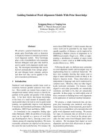
Input: initial parameters α
(0)
, observed data x,
annealing schedule
˜

r
: N → 2

r
Output: learned parameters α and approximate
posterior q(θ, y)
t ← 1;
repeat
E-step: repeat
E-step: forall i ∈ [r] do: q

(t+1)
i
(y) ← argmax
q(y)∈Q
i
F

(
P
j=i
λ
j
q
(t)
i
(θ)q(y) + λ
i
q
(t)
i
q(y ), α
(t)
)
M-step: forall i ∈ [r] do: q
(t+1)
i
(θ) ← argmax
q(θ)∈Q
i
F


(
P
j=i
λ
j
q(θ)q
(t)
i
(y) + λ
i
q
(t)
i
q(y ), α
(t)
)
C-step: λ
(t+1)
←
argmax
λ∈
˜

r
(t)
F

(
P

r
j=1
λ
j
q
(t)
i
(θ)q
(t)
i
(y), α
(t)
)
until convergence ;
M-step: α
(t+1)
←
argmax
α
F

(
P
r
i=1
λ
i
q
(t+1)
i

(θ)q
(t+1)
i
(y), α)
t ← t + 1;
until convergence ;
return α
(t)
,
P
r
i=1
λ
i
q
(t)
i
(θ)q
(t)
i
(y)
Figure 1: The constrained variational mixture EM algorithm.
[n] denotes {1, , n}.
2.2 Tractability
We now turn to further alterations of the bound in
Eq. 2 to make it more tractable. The main problem
is the entropy term which is not easy to compute,
because it includes a log term over a mixture of
distributions from Q
i

. We require the distributions
in Q
i
to factorize over the hidden structure y, but
this only helps with the first term in Eq. 2.
We note that because the entropy function is
convex, we can get a lower bound on H(q):
H(q) ≥

r
i=1
λ
i
H(q
i
) =

r
i=1
λ
i
H(q
i
(θ, y))
Substituting the modified entropy term into
Eq. 2 still yields a lower bound on the likeli-
hood. This change makes the E-step tractable,
because each distribution q
i
(y) can be computed

separately by optimizing a bound which depends
only on the variational parameters in that distribu-
tion. In fact, the bound on the left hand side in
Proposition 1 becomes the function that we opti-
mize instead of G(q, α).
Without proper constraints, the λ update can be
intractable as well. It requires maximizing a lin-
ear objective (in λ) while constraining the λ to
be from a particular subspace of the probability
simplex,
˜

r
(t). To solve this issue, we require
that
˜

r
(t) is polyhedral, making it possible to ap-
ply linear programming (Boyd and Vandenberghe,
2004).
The bound we optimize is:
2
F


r

i=1
λ

i
q
i
(θ, y), α

(8)
=
r

i=1
λ
i

E
q
i
(θ,y)
[log p(θ, y, x | m)] + H(q
i
(θ, y))

with λ ∈
˜

r
(t
final
) and (q
i
(θ, y)) ∈ Q

i
. The
algorithm for optimizing this bound is in Fig. 1,
which includes an extra M-step to optimize α (see
extended report).
3 Experiments
We tested our method on the unsupervised learn-
ing problem of dependency grammar induction.
For the generative model, we used the dependency
model with valence as it appears in Klein and Man-
ning (2004). We used the data from the Chi-
nese treebank (Xue et al., 2004). Following stan-
dard practice, sentences were stripped of words
and punctuation, leaving part-of-speech tags for
the unsupervised induction of dependency struc-
ture, and sentences of length more than 10 were
removed from the set. We experimented with
a Dirichlet prior over the parameters and logis-
tic normal priors over the parameters, and found
the latter to still be favorable with our method, as
in Cohen et al. (2008). We therefore report results
with our method only for the logistic normal prior.
We do inference on sections 1–270 and 301–1151
of CTB10 (4,909 sentences) by running the EM al-
gorithm for 20 iterations, for which all algorithms
have their variational bound converge.
To evaluate performance, we report the fraction
of words whose predicted parent matches the gold
standard (attachment accuracy). For parsing, we
use the minimum Bayes risk parse.

Our mixture components Q
i
are based on simple
linguistic tendencies of Chinese syntax. These ob-
servations include the tendency of dependencies to
(a) emanate from the right of the current position
and (b) connect words which are nearby (in string
distance). We experiment with six mixture com-
ponents: (1) RIGHTATTACH: Each word’s parent
is to the word’s right. The root, therefore, is al-
ways the rightmost word; (2) ALLRIGHT: The
rightmost word is the parent of all positions in the
sentence (there is only one such tree); (3) LEFT-
CHAIN: The tree forms a chain, such that each
2
This is a less tight bound than the one in Bishop et al.
(1998), but it is easier to handle computationally.
3
learning setting
LEFTCHAIN 34.9
vanilla EM 38.3
LN, mean-field 48.9
This paper: I II III
RIGHTATTACH 49.1 47.1 49.8
ALLRIGHT 49.4 49.4 48.4
LEFTCHAIN 47.9 46.5 49.9
VERBASROOT 50.5 50.2 49.4
NOUNSEQUE NCE 48.9 48.9 49.9
SHORTDEP 49.5 48.4 48.4
RA+VAR+SD 50.5 50.6 50.1

Table 1: Results (attachment accuracy). The baselines are
LEFTCHAIN as a parsing model (attaches each word to the
word on its right), non-Bayesian EM, and mean-field vari-
ational EM without any constraints. These are compared
against the six mixture components mentioned in the text. (I)
corresponds to simplex annealing experiments (λ
(0)
1
= 0.85);
(II–III) correspond to fixed values, 0.85 and 0.95, for the
mixture coefficients. With the last row, λ
2
to λ
4
are always
(1 − λ
1
)/3. Boldface denotes the best result in each row.
word is governed by the word to its right; (4) VER-
BASROOT: Only verbs can attach to the wall node
$; (5) NOUNSEQUENCE: Every sequence of n NN
(nouns) is assumed to be a noun phrase, hence the
first n −1 NNs are attached to the last NN; and (6)
SHORTDEP: Allow only dependencies of length
four or less. This is a strict model reminiscent
of the successful application of structural bias to
grammar induction (Smith and Eisner, 2006).
These components are added to a variational
DMV model without the sum-to-1 constraint on
θ. This complements variational techniques which

state that the optimal solution during the E-step
for the mean-field variational EM algorithm is a
weighted grammar of the same form of p(x, y | θ)
(DMV in our case). Using the mixture compo-
nents this way has the effect of smoothing the esti-
mated grammar event counts during the E-step, in
the direction of some prior expectations.
Let λ
1
correspond to the component of the orig-
inal DMV model, and let λ
2
correspond to one of
the components from the above list. Variational
techniques show that if we let λ
1
obtain the value
1, then the optimal solution will be λ
1
= 1 and
λ
2
= 0. We therefore restrict λ
1
to be smaller than
1. More specifically, we use an annealing process
which starts by limiting λ
1
to be ≤ s = 0.85 (and
hence limits λ

2
to be ≥ 0.15) and increases s at
each step by 1% until s reaches 0.95. In addition,
we also ran the algorithm with λ
1
fixed at 0.85 and
λ
1
fixed at 0.95 to check the effectiveness of an-
nealing on the simplex.
Table 1 describes the results of our experi-
ments. In general, using additional mixture com-
ponents has a clear advantage over the mean-field
assumption. The best result with a single mix-
ture is achieved with annealing, and the VERBAS-
ROOT component. A combination of the mix-
tures (RIGHTATTACH) together with VERBAS-
ROOT and SHORTDEP led to an additional im-
provement, implying that proper selection of sev-
eral mixture components together can achieve a
performance gain.
4 Conclusion
We described a variational EM algorithm that uses
a mixture model for the variational model. We
refined the algorithm with an annealing mecha-
nism to avoid local maxima. We demonstrated
the effectiveness of the algorithm on a dependency
grammar induction task. Our results show that
with a good choice of mixture components and
annealing schedule, we achieve improvements for

this task over mean-field variational inference.
References
M. J. Beal and Z. Gharamani. 2003. The variational
Bayesian EM algorithm for incomplete data: with appli-
cation to scoring graphical model structures. In Proc. of
Bayesian Statistics.
C. Bishop, N. Lawrence, T. S. Jaakkola, and M. I. Jordan.
1998. Approximating posterior distributions in belief net-
works using mixtures. In Advances in NIPS.
C. M. Bishop. 2006. Pattern Recognition and Machine
Learning. Springer.
S. Boyd and L. Vandenberghe. 2004. Convex Optimization.
Cambridge Press.
S. B. Cohen and N. A. Smith. 2009. Variational inference
with prior knowledge. Technical report, Carnegie Mellon
University.
S. B. Cohen, K. Gimpel, and N. A. Smith. 2008. Logis-
tic normal priors for unsupervised probabilistic grammar
induction. In Advances in NIPS.
J. V. Grac¸a, K. Ganchev, and B. Taskar. 2007. Expectation
maximization and posterior constraints. In Advances in
NIPS.
D. Klein and C. D. Manning. 2004. Corpus-based induction
of syntactic structure: Models of dependency and con-
stituency. In Proc. of ACL.
F. C. N. Pereira and Y. Schabes. 1992. Inside-outside reesti-
mation from partially bracketed corpora. In Proc. of ACL.
K. Rose, E. Gurewitz, and G. C. Fox. 1990. Statistical me-
chanics and phrase transitions in clustering. Physical Re-
view Letters, 65(8):945–948.

N. A. Smith and J. Eisner. 2006. Annealing structural bias
in multilingual weighted grammar induction. In Proc. of
COLING-ACL.
N. Xue, F. Xia, F D. Chiou, and M. Palmer. 2004. The Penn
Chinese Treebank: Phrase structure annotation of a large
corpus. Natural Language Engineering, 10(4):1–30.
4