Báo cáo khoa học: "A Bayesian Model for Discovering Typological Implications" ppt
Bạn đang xem bản rút gọn của tài liệu. Xem và tải ngay bản đầy đủ của tài liệu tại đây (316.22 KB, 8 trang )
Proceedings of the 45th Annual Meeting of the Association of Computational Linguistics, pages 65–72,
Prague, Czech Republic, June 2007.
c
2007 Association for Computational Linguistics
A Bayesian Model for Discovering Typological Implications
Hal Daum
´
e III
School of Computing
University of Utah
Lyle Campbell
Department of Linguistics
University of Utah
Abstract
A standard form of analysis for linguis-
tic typology is the universal implication.
These implications state facts about the
range of extant languages, such as “if ob-
jects come after verbs, then adjectives come
after nouns.” Such implications are typi-
cally discovered by painstaking hand anal-
ysis over a small sample of languages. We
propose a computational model for assist-
ing at this process. Our model is able to
discover both well-known implications as
well as some novel implications that deserve
further study. Moreover, through a careful
application of hierarchical analysis, we are
able to cope with the well-known sampling
problem: languages are not independent.
1 Introduction
Linguistic typology aims to distinguish between log-
ically possible languages and actually observed lan-
guages. A fundamental building block for such an
understanding is the universal implication (Green-
berg, 1963). These are short statements that restrict
the space of languages in a concrete way (for in-
stance “object-verb ordering implies adjective-noun
ordering”); Croft (2003), Hawkins (1983) and Song
(2001) provide excellent introductions to linguistic
typology. We present a statistical model for auto-
matically discovering such implications from a large
typological database (Haspelmath et al., 2005).
Analyses of universal implications are typically
performed by linguists, inspecting an array of 30-
100 languages and a few pairs of features. Looking
at all pairs of features (typically several hundred) is
virtually impossible by hand. Moreover, it is insuf-
ficient to simply look at counts. For instance, results
presented in the form “verb precedes object implies
prepositions in 16/19 languages” are nonconclusive.
While compelling, this is not enough evidence to de-
cide if this is a statistically well-founded implica-
tion. For one, maybe 99% of languages have prepo-
sitions: then the fact that we’ve achieved a rate of
84% actually seems really bad. Moreover, if the 16
languages are highly related historically or areally
(geographically), and the other 3 are not, then we
may have only learned something about geography.
In this work, we propose a statistical model that
deals cleanly with these difficulties. By building a
computational model, it is possible to apply it to
a very large typological database and search over
many thousands of pairs of features. Our model
hinges on two novel components: a statistical noise
model a hierarchical inference over language fam-
ilies. To our knowledge, there is no prior work
directly in this area. The closest work is repre-
sented by the books Possible and Probable Lan-
guages (Newmeyer, 2005) and Language Classifica-
tion by Numbers (McMahon and McMahon, 2005),
but the focus of these books is on automatically dis-
covering phylogenetic trees for languages based on
Indo-European cognate sets (Dyen et al., 1992).
2 Data
The database on which we perform our analysis is
the World Atlas of Language Structures (Haspel-
math et al., 2005). This database contains infor-
mation about 2150 languages (sampled from across
the world; Figure 1 depicts the locations of lan-
65
Numeral Glottalized Number of
Language Classifiers Rel/N Order O/V Order Consonants Tone Genders
English Absent NRel VO None None Three
Hindi Absent RelN OV None None Two
Mandarin Obligatory RelN VO None Complex None
Russian Absent NRel VO None None Three
Tukang Besi Absent ? Either Implosives None Three
Zulu Absent NRel VO Ejectives Simple Five+
Table 1: Example database entries for a selection of diverse languages and features.
−150 −100 −50 0 50 100 150
−40
−20
0
20
40
60
Figure 1: Map of the 2150 languages in the database.
guages). There are 139 features in this database,
broken down into categories such as “Nominal Cate-
gories,” “Simple Clauses,” “Phonology,” “Word Or-
der,” etc. The database is sparse: for many lan-
guage/feature pairs, the feature value is unknown. In
fact, only about 16% of all possible language/feature
pairs are known. A sample of five languages and six
features from the database are shown in Table 1.
Importantly, the density of samples is not random.
For certain languages (eg., English, Chinese, Rus-
sian), nearly all features are known, whereas other
languages (eg., Asturian, Omagua, Frisian) that have
fewer than five feature values known. Furthermore,
some features are known for many languages. This
is due to the fact that certain features take less effort
to identify than others. Identifying, for instance, if
a language has a particular set of phonological fea-
tures (such as glottalized consonants) requires only
listening to speakers. Other features, such as deter-
mining the order of relative clauses and nouns re-
quire understanding much more of the language.
3 Models
In this section, we propose two models for automat-
ically uncovering universal implications from noisy,
sparse data. First, note that even well attested impli-
cations are not always exceptionless. A common ex-
ample is that verbs preceding objects (“VO”) implies
adjectives following nouns (“NA”). This implication
(VO ⊃ NA) has one glaring exception: English.
This is one particular form of noise. Another source
of noise stems from transcription. WALS contains
data about languages documented by field linguists
as early as the 1900s. Much of this older data was
collected before there was significant agreement in
documentation style. Different field linguists of-
ten had different dimensions along which they seg-
mented language features into classes. This leads to
noise in the properties of individual languages.
Another difficulty stems from the sampling prob-
lem. This is a well-documented issue (see, eg.,
(Croft, 2003)) stemming from the fact that any set of
languages is not sampled uniformly from the space
of all probable languages. Politically interesting
languages (eg., Indo-European) and typologically
unusual languages (eg., Dyirbal) are better docu-
mented than others. Moreover, languages are not in-
dependent: German and Dutch are more similar than
German and Hindi due to history and geography.
The first model, FLAT, treats each language as in-
dependent. It is thus susceptible to sampling prob-
lems. For instance, the WALS database contains a
half dozen versions of German. The FLAT model
considers these versions of German just as statisti-
cally independent as, say, German and Hindi. To
cope with this problem, we then augment the FLAT
model into a HIERarchical model that takes advan-
tage of known hierarchies in linguistic phylogenet-
ics. The HIER model explicitly models the fact that
individual languages are not independent and exhibit
strong familial dependencies. In both models, we
initially restrict our attention to pairs of features. We
will describe our models as if all features are binary.
We expand any multi-valued feature with K values
into K binary features in a “one versus rest” manner.
3.1 The FLAT Model
In the FLAT model, we consider a 2 × N matrix of
feature values. The N corresponds to the number of
languages, while the 2 corresponds to the two fea-
tures currently under consideration (eg., object/verb
order and noun/adjective order). The order of the
66
two features is important: f
1
implies f
2
is logically
different from f
2
implies f
1
. Some of the entries in
the matrix will be unknown. We may safely remove
all languages from consideration for which both are
unknown, but we do not remove languages for which
only one is unknown. We do so because our model
needs to capture the fact that if f
2
is always true,
then f
1
⊃ f
2
is uninteresting.
The statistical model is set up as follows. There is
a single variable (we will denote this variable “m”)
corresponding to whether the implication holds.
Thus, m = 1 means that f
1
implies f
2
and m = 0
means that it does not. Independent of m, we specify
two feature priors, π
1
and π
2
for f
1
and f
2
respec-
tively. π
1
specifies the prior probability that f
1
will
be true, and π
2
specifies the prior probability that f
2
will be true. One can then put the model together
na
¨
ıvely as follows. If m = 0 (i.e., the implication
does not hold), then the entire data matrix is gener-
ated by choosing values for f
1
(resp., f
2
) indepen-
dently according to the prior probability π
1
(resp.,
π
2
). On the other hand, if m = 1 (i.e., the impli-
cation does hold), then the first column of the data
matrix is generated by choosing values for f
1
inde-
pendently by π
1
, but the second column is generated
differently. In particular, if for a particular language,
we have that f
1
is true, then the fact that the implica-
tion holds means that f
2
must be true. On the other
hand, if f
1
is false for a particular language, then we
may generate f
2
according to the prior probability
π
2
. Thus, having m = 1 means that the model is
significantly more constrained. In equations:
p(f
1
| π
1
) = π
f
1
1
(1 − π
1
)
1−f
1
p(f
2
| f
1
, π
2
, m) =
f
2
m = f
1
= 1
π
f
2
2
(1 − π
2
)
1−f
2
otherwise
The problem with this na
¨
ıve model is that it does
not take into account the fact that there is “noise”
in the data. (By noise, we refer either to mis-
annotations, or to “strange” languages like English.)
To account for this, we introduce a simple noise
model. There are several options for parameteriz-
ing the noise, depending on what independence as-
sumptions we wish to make. One could simply spec-
ify a noise rate for the entire data set. One could
alternatively specify a language-specific noise rate.
Or one could specify a feature-specific noise rate.
We opt for a blend between the first and second op-
Figure 2: Graphical model for the FLAT model.
tion. We assume an underlying noise rate for the en-
tire data set, but that, conditioned on this underlying
rate, there is a language-specific noise level. We be-
lieve this to be an appropriate noise model because it
models the fact that the majority of information for
a single language is from a single source. Thus, if
there is an error in the database, it is more likely that
other errors will be for the same languages.
In order to model this statistically, we assume that
there are latent variables e
1,n
and e
2,n
for each lan-
guage n. If e
1,n
= 1, then the first feature for lan-
guage n is wrong. Similarly, if e
2,n
= 1, then the
second feature for language n is wrong. Given this
model, the probabilities are exactly as in the na
¨
ıve
model, with the exception that instead of using f
1
(resp., f
2
), we use the exclusive-or
1
f
1
⊗ e
1
(resp.,
f
2
⊗ e
2
) so that the feature values are flipped when-
ever the noise model suggests an error.
The graphical model for the FLAT model is shown
in Figure 2. Circular nodes denote random variables
and arrows denote conditional dependencies. The
rectangular plate denotes the fact that the elements
contained within it are replicated N times (N is the
number of languages). In this model, there are four
“root” nodes: the implication value m; the two fea-
ture prior probabilities π
1
and π
2
; and the language-
specific error rate ǫ. On all of these nodes we place
Bayesian priors. Since m is a binary random vari-
able, we place a Bernoulli prior on it. The πs are
Bernoulli random variables, so they are given inde-
pendent Beta priors. Finally, the noise rate ǫ is also
given a Beta prior. For the two Beta parameters gov-
erning the error rate (i.e., a
ǫ
and b
ǫ
) we set these by
hand so that the mean expected error rate is 5% and
the probability of the error rate being between 0%
and 10% is 50% (this number is based on an expert
opinion of the noise-rate in the data). For the rest of
1
The exclusive-or of a and b, written a ⊗ b, is true exactly
when either a or b is true but not both.
67
the parameters we use uniform priors.
3.2 The HIER Model
A significant difficulty in working with any large ty-
pological database is that the languages will be sam-
pled nonuniformly. In our case, this means that im-
plications that seem true in the FLAT model may
only be true for, say, Indo-European, and the remain-
ing languages are considered noise. While this may
be interesting in its own right, we are more interested
in discovering implications that are truly universal.
We model this using a hierarchical Bayesian
model. In essence, we take the FLAT model and
build a notion of language relatedness into it. In
particular, we enforce a hierarchy on the m impli-
cation variables. For simplicity, suppose that our
“hierarchy” of languages is nearly flat. Of the N
languages, half of them are Indo-European and the
other half are Austronesian. We will use a nearly
identical model to the FLAT model, but instead of
having a single m variable, we have three: one for
IE, one for Austronesian and one for “all languages.”
For a general tree, we assign one implication vari-
able for each node (including the root and leaves).
The goal of the inference is to infer the value of the
m variable corresponding to the root of the tree.
All that is left to specify the full HIER model
is to specify the probability distribution of the m
random variables. We do this as follows. We
place a zero mean Gaussian prior with (unknown)
variance σ
2
on the root m. Then, for a non-root
node, we use a Gaussian with mean equal to the
“m” value of the parent and tied variance σ
2
. In
our three-node example, this means that the root is
distributed Nor(0, σ
2
) and each child is distributed
Nor(m
root
, σ
2
), where m
root
is the random variable
corresponding to the root. Finally, the leaves (cor-
responding to the languages themselves) are dis-
tributed logistic-binomial. Thus, the m random vari-
able corresponding to a leaf (language) is distributed
Bin(s(m
par
)), where m
par
is the m value for the par-
ent (internal) node and s is the sigmoid function
s(x) = [1 + exp(−x)]
−1
.
The intuition behind this model is that the m value
at each node in the tree (where a node is either “all
languages” or a specific language family or an in-
dividual language) specifies the extent to which the
implication under consideration holds for that node.
A large positive m means that the implication is very
likely to hold. A large negative value means it is
very likely to not hold. The normal distributions
across edges in the tree indicate that we expect the
m values not to change too much across the tree. At
the leaves (i.e., individual languages), the logistic-
binomial simply transforms the real-valued ms into
the range [0, 1] so as to make an appropriate input to
the binomial distribution.
4 Statistical Inference
In this section, we describe how we use Markov
chain Monte Carlo methods to perform inference
in the statistical models described in the previous
section; Andrieu et al. (2003) provide an excel-
lent introduction to MCMC techniques. The key
idea behind MCMC techniques is to approximate in-
tractable expectations by drawing random samples
from the probability distribution of interest. The ex-
pectation can then be approximated by an empirical
expectation over these sample.
For the FLAT model, we use a combination of
Gibbs sampling with rejection sampling as a sub-
routine. Essentially, all sampling steps are standard
Gibbs steps, except for sampling the error rates e.
The Gibbs step is not available analytically for these.
Hence, we use rejection sampling (drawing from the
Beta prior and accepting according to the posterior).
The sampling procedure for the HIER model is
only slightly more complicated. Instead of perform-
ing a simple Gibbs sample for m in Step (4), we
first sample the m values for the internal nodes us-
ing simple Gibbs updates. For the leaf nodes, we
use rejection sampling. For this rejection, we draw
proposal values from the Gaussian specified by the
parent m, and compute acceptance probabilities.
In all cases, we run the outer Gibbs sampler for
1000 iterations and each rejection sampler for 20 it-
erations. We compute the marginal values for the m
implication variables by averaging the sampled val-
ues after dropping 200 “burn-in” iterations.
5 Data Preprocessing and Search
After extracting the raw data from the WALS elec-
tronic database (Haspelmath et al., 2005)
2
, we per-
form a minor amount of preprocessing. Essen-
tially, we have manually removed certain feature
2
This is nontrivial—we are currently exploring the possibil-
ity of freely sharing these data.
68
values from the database because they are underrep-
resented. For instance, the “Glottalized Consonants”
feature has eight possible values (one for “none”
and seven for different varieties of glottalized conso-
nants). We reduce this to simply two values “has” or
“has not.” 313 languages have no glottalized conso-
nants and 139 have some variety of glottalized con-
sonant. We have done something similar with ap-
proximately twenty of the features.
For the HIER model, we obtain the hierarchy in
one of two ways. The first hierarchy we use is the
“linguistic hierarchy” specified as part of the WALS
data. This hierarchy divides languages into families
and subfamilies. This leads to a tree with the leaves
at depth four. The root has 38 immediate children
(corresponding to the major families), and there are
a total of 314 internal nodes. The second hierar-
chy we use is an areal hierarchy obtained by clus-
tering languages according to their latitude and lon-
gitude. For the clustering we first cluster all the lan-
guages into 6 “macro-clusters.” We then cluster each
macro-cluster individually into 25 “micro-clusters.”
These micro-clusters then have the languages at their
leaves. This yields a tree with 31 internal nodes.
Given the database (which contains approxi-
mately 140 features), performing a raw search even
over all possible pairs of features would lead to over
19, 000 computations. In order to reduce this space
to a more manageable number, we filter:
• There must be at least 250 languages for which both fea-
tures are known.
• There must be at least 15 languages for which both fea-
ture values hold simultaneously.
• Whenever f
1
is true, at least half of the languages also
have f
2
true.
Performing all these filtration steps reduces the
number of pairs under consideration to 3442. While
this remains a computationally expensive procedure,
we were able to perform all the implication compu-
tations for these 3442 possible pairs in about a week
on a single modern machine (in Matlab).
6 Results
The task of discovering universal implications is, at
its heart, a data-mining task. As such, it is difficult
to evaluate, since we often do not know the correct
answers! If our model only found well-documented
implications, this would be interesting but useless
from the perspective of aiding linguists focus their
energies on new, plausible implications. In this sec-
tion, we present the results of our method, together
with both a quantitative and qualitative evaluation.
6.1 Quantitative Evaluation
In this section, we perform a quantitative evaluation
of the results based on predictive power. That is,
one generally would prefer a system that finds im-
plications that hold with high probability across the
data. The word “generally” is important: this qual-
ity is neither necessary nor sufficient for the model
to be good. For instance, finding 1000 implications
of the form A
1
⊃ X, A
2
⊃ X, . . . , A
1000
⊃ X is
completely uninteresting if X is true in 99% of the
cases. Similarly, suppose that a model can find 1000
implications of the form X ⊃ A
1
, . . . , X ⊃ A
1000
,
but X is only true in five languages. In both of these
cases, according to a “predictive power” measure,
these would be ideal systems. But they are both
somewhat uninteresting.
Despite these difficulties with a predictive power-
based evaluation, we feel that it is a good way to un-
derstand the relative merits of our different models.
Thus, we compare the following systems: FLAT (our
proposed flat model), LINGHIER (our model using
the phylogenetic hierarchy), DISTHIER (our model
using the areal hierarchy) and RANDOM (a model
that ranks implications—that meet the three qualifi-
cations from the previous section—randomly).
The models are scored as follows. We take the
entire WALS data set and “hide” a random 10%
of the entries. We then perform full inference and
ask the inferred model to predict the missing val-
ues. The accuracy of the model is the accuracy of
its predictions. To obtain a sense of the quality of
the ranking, we perform this computation on the
top k ranked implications provided by each model;
k ∈ {2, 4, 8, . . . , 512, 1024}.
The results of this quantitative evaluation are
shown in Figure 3 (on a log-scale for the x-axis).
The two best-performing models are the two hier-
archical models. The flat model does significantly
worse and the random model does terribly. The ver-
tical lines are a standard deviation over 100 folds of
the experiment (hiding a different 10% each time).
The difference between the two hierarchical mod-
els is typically not statistically significant. At the
top of the ranking, the model based on phylogenetic
69
0 1 2 3 4 5 6 7 8 9 10
0.65
0.7
0.75
0.8
0.85
0.9
0.95
1
Number of Implications (log
2
)
Prediction Accuracy
LingHier DistHier Flat Random
Figure 3: Results of quantitative (predictive) evalua-
tion. Top curves are the hierarchical models; middle
is the flat model; bottom is the random baseline.
information performs marginally better; at the bot-
tom of the ranking, the order flips. Comparing the
hierarchical models to the flat model, we see that
adequately modeling the a priori similarity between
languages is quite important.
6.2 Cross-model Comparison
The results in the previous section support the con-
clusion that the two hierarchical models are doing
something significantly different (and better) than
the flat model. This clearly must be the case. The
results, however, do not say whether the two hierar-
chies are substantially different. Moreover, are the
results that they produce substantially different. The
answer to these two questions is “yes.”
We first address the issue of tree similarity. We
consider all pairs of languages which are at distance
0 in the areal tree (i.e., have the same parent). We
then look at the mean tree-distance between those
languages in the phylogenetic tree. We do this for all
distances in the areal tree (because of its construc-
tion, there are only three: 0, 2 and 4). The mean
distances in the phylogenetic tree corresponding to
these three distances in the areal tree are: 2.9, 3.5
and 4.0, respectively. This means that languages that
are “nearby” in the areal tree are quite often very far
apart in the phylogenetic tree.
To answer the issue of whether the results ob-
tained by the two trees are similar, we employ
Kendall’s τ statistic. Given two ordered lists, the
τ statistic computes how correlated they are. τ is
always between 0 and 1, with 1 indicating identical
ordering and 0 indicated completely reversed order-
ing. The results are as follows. Comparing FLAT
to LINGHIER yield τ = 0.4144, a very low correla-
tion. Between FLAT and DISTHIER, τ = 0.5213,
also very low. These two are as expected. Fi-
nally, between LINGHIER and DISTHIER, we ob-
tain τ = 0.5369, a very low correlation, considering
that both perform well predictively.
6.3 Qualitative Analysis
For the purpose of a qualitative analysis, we re-
produce the top 30 implications discovered by the
LINGHIER model in Table 2 (see the final page).
3
Each implication is numbered, then the actual im-
plication is presented. For instance, #7 says that
any language that has adjectives preceding their
governing nouns also has numerals preceding their
nouns. We additionally provide an “analysis” of
many of these discovered implications. Many of
them (eg., #7) are well known in the typological lit-
erature. These are simply numbered according to
well-known references. For instance our #7 is im-
plication #18 from Greenberg, reproduced by Song
(2001). Those that reference Hawkins (eg., #11) are
based on implications described by Hawkins (1983);
those that reference Lehmann are references to the
principles decided by Lehmann (1981) in Ch 4 & 8.
Some of the implications our model discovers
are obtained by composition of well-known implica-
tions. For instance, our #3 (namely, OV ⊃ Genitive-
Noun) can be obtained by combining Greenberg #4
(OV ⊃ Postpositions) and Greenberg #2a (Postpo-
sitions ⊃ Genitive-Noun). It is quite encouraging
that 14 of our top 21 discovered implications are
well-known in the literature (and this, not even con-
sidering the tautalogically true implications)! This
strongly suggests that our model is doing something
reasonable and that there is true structure in the data.
In addition to many of the known implications
found by our model, there are many that are “un-
known.” Space precludes attempting explanations
of them all, so we focus on a few. Some are easy.
Consider #8 (Strongly suffixing ⊃ Tense-aspect suf-
fixes): this is quite plausible—if you have a lan-
3
In truth, our model discovers several tautalogical implica-
tions that we have removed by hand before presentation. These
are examples like “SVO ⊃ VO” or “No unusual consonants ⊃
no glottalized consonants.” It is, of course, good that our model
discovers these, since they are obviously true. However, to save
space, we have withheld them from presentation here. The 30th
implication presented here is actually the 83rd in our full list.
70
guage that tends to have suffixes, it will probably
have suffixes for tense/aspect. Similarly, #10 states
that languages with verb morphology for questions
lack question particles; again, this can be easily ex-
plained by an appeal to economy.
Some of the discovered implications require a
more involved explanation. One such example is
#20: labial-velars implies no uvulars.
4
It turns out
that labial-velars are most common in Africa just
north of the equator, which is also a place that has
very few uvulars (there are a handful of other ex-
amples, mostly in Papua New Guinea). While this
implication has not been previously investigated, it
makes some sense: if a language has one form of
rare consonant, it is unlikely to have another.
As another example, consider #28: Obligatory
suffix pronouns implies no possessive affixes. This
means is that in languages (like English) for which
pro-drop is impossible, possession is not marked
morphologically on the head noun (like English,
“book” appears the same regarless of if it is “his
book” or “the book”). This also makes sense: if you
cannot drop pronouns, then one usually will mark
possession on the pronoun, not the head noun. Thus,
you do not need marking on the head noun.
Finally, consider #25: High and mid front vowels
(i.e., / u/, etc.) implies large vowel inventory (≥ 7
vowels). This is supported by typological evidence
that high and mid front vowels are the “last” vowels
to be added to a language’s repertoire. Thus, in order
to get them, you must also have many other types of
vowels already, leading to a large vowel inventory.
Not all examples admit a simple explanation and
are worthy of further thought. Some of which (like
the ones predicated on “SV”) may just be peculiar-
ities of the annotation style: the subject verb order
changes frequently between transitive and intransi-
tive usages in many languages, and the annotation
reflects just one. Some others are bizzarre: why not
having fricatives should mean that you don’t have
tones (#27) is not a priori clear.
6.4 Multi-conditional Implications
Many implications in the literature have multiple
implicants. For instance, much research has gone
4
Labial-velars and uvulars are rare consonants (order 100
languages). Labial-velars are joined sounds like /kp/ and /gb/
(to English speakers, sounding like chicken noises); uvulars
sounds are made in the back of the throat, like snoring.
Implicants Implicand
Postpositions
⊃ Demonstrative-Noun
Adjective-Noun
Posessive prefixes
⊃ Genitive-Noun
Tense-aspect suffixes
Case suffixes
⊃ Genitive-Noun
Plural suffix
Adjective-Noun
⊃ OV
Genitive-Noun
High cons/vowel ratio
⊃ No tones
No front-rounded vowels
Negative affix
⊃ OV
Genitive-Noun
No front-rounded vowels
⊃ Large vowel quality inventory
Labial velars
Subordinating suffix
⊃ Postpositions
Tense-aspect suffixes
No case affixes
⊃ Initial subordinator word
Prepositions
Strongly suffixing
⊃ Genitive-Noun
Plural suffix
Table 3: Top implications discovered by the
LINGHIER multi-conditional model.
into looking at which implications hold, considering
only “VO” languages, or considering only languages
with prepositions. It is straightforward to modify
our model so that it searches over triples of features,
conditioning on two and predicting the third. Space
precludes an in-depth discussion of these results, but
we present the top examples in Table 3 (after remov-
ing the tautalogically true examples, which are more
numerous in this case, as well as examples that are
directly obtainable from Table 2). It is encouraging
that in the top 1000 multi-conditional implications
found, the most frequently used were “OV” (176
times) “Postpositions” (157 times) and “Adjective-
Noun” (89 times). This result agrees with intuition.
7 Discussion
We have presented a Bayesian model for discovering
universal linguistic implications from a typological
database. Our model is able to account for noise in
a linguistically plausible manner. Our hierarchical
models deal with the sampling issue in a unique way,
by using prior knowledge about language families to
“group” related languages. Quantitatively, the hier-
archical information turns out to be quite useful, re-
gardless of whether it is phylogenetically- or areally-
based. Qualitatively, our model can recover many
well-known implications as well as many more po-
tential implications that can be the object of future
linguistic study. We believe that our model is suf-
71
# Implicant ⊃ Implicand Analysis
1 Postpositions ⊃ Genitive-Noun Greenberg #2a
2 OV ⊃ Postpositions Greenberg #4
3 OV ⊃ Genitive-Noun Greenberg #4 + Greenberg #2a
4 Genitive-Noun ⊃ Postpositions Greenberg #2a (converse)
5 Postpositions ⊃ OV Greenberg #2b (converse)
6 SV ⊃ Genitive-Noun ???
7 Adjective-Noun ⊃ Numeral-Noun Greenberg #18
8 Strongly suffixing ⊃ Tense-aspect suffixes Clear explanation
9 VO ⊃ Noun-Relative Clause Lehmann
10 Interrogative verb morph ⊃ No question particle Appeal to economy
11 Numeral-Noun ⊃ Demonstrative-Noun Hawkins XVI (for postpositional languages)
12 Prepositions ⊃ VO Greenberg #3 (converse)
13 Adjective-Noun ⊃ Demonstrative-Noun Greenberg #18
14 Noun-Adjective ⊃ Postpositions Lehmann
15 SV ⊃ Postpositions ???
16 VO ⊃ Prepositions Greenberg #3
17 Initial subordinator word ⊃ Prepositions Operator-operand principle (Lehmann)
18 Strong prefixing ⊃ Prepositions Greenberg #27b
19 Little affixation ⊃ Noun-Adjective ???
20 Labial-velars ⊃ No uvular consonants See text
21 Negative word ⊃ No pronominal possessive affixes See text
22 Strong prefixing ⊃ VO Lehmann
23 Subordinating suffix ⊃ Strongly suffixing ???
24 Final subordinator word ⊃ Postpositions Operator-operand principle (Lehmann)
25 High and mid front vowels ⊃ Large vowel inventories See text
26 Plural prefix ⊃ Noun-Genitive ???
27 No fricatives ⊃ No tones ???
28 Obligatory subject pronouns ⊃ No pronominal possessive affixes See text
29 Demonstrative-Noun ⊃ Tense-aspect suffixes Operator-operand principle (Lehmann)
30 Prepositions ⊃ Noun-Relative clause Lehmann, Hawkins
Table 2: Top 30 implications discovered by the LINGHIER model.
ficiently general that it could be applied to many
different typological databases — we attempted not
to “overfit” it to WALS. Our hope is that the au-
tomatic discovery of such implications not only
aid typologically-inclined linguists, but also other
groups. For instance, well-attested universal impli-
cations have the potential to reduce the amount of
data field linguists need to collect. They have also
been used computationally to aid in the learning of
unsupervised part of speech taggers (Schone and Ju-
rafsky, 2001). Many extensions are possible to this
model; for instance attempting to uncover typolog-
ically hierarchies and other higher-order structures.
We have made the full output of all models available
at e/WALS.
Acknowledgments. We are grateful to Yee Whye
Teh, Eric Xing and three anonymous reviewers for
their feedback on this work.
References
Christophe Andrieu, Nando de Freitas, Arnaud Doucet, and
Michael I. Jordan. 2003. An introduction to MCMC for
machine learning. Machine Learning (ML), 50:5–43.
William Croft. 2003. Typology and Univerals. Cambridge
University Press.
Isidore Dyen, Joseph Kurskal, and Paul Black. 1992. An
Indoeuropean classification: A lexicostatistical experiment.
Transactions of the American Philosophical Society, 82(5).
American Philosophical Society.
Joseph Greenberg, editor. 1963. Universals of Languages.
MIT Press.
Martin Haspelmath, Matthew Dryer, David Gil, and Bernard
Comrie, editors. 2005. The World Atlas of Language Struc-
tures. Oxford University Press.
John A. Hawkins. 1983. Word Order Universals: Quantitative
analyses of linguistic structure. Academic Press.
Winfred Lehmann, editor. 1981. Syntactic Typology, volume
xiv. University of Texas Press.
April McMahon and Robert McMahon. 2005. Language Clas-
sification by Numbers. Oxford University Press.
Frederick J. Newmeyer. 2005. Possible and Probable Lan-
guages: A Generative Perspective on Linguistic Typology.
Oxford University Press.
Patrick Schone and Dan Jurafsky. 2001 Language Independent
Induction of Part of Speech Class Labels Using only Lan-
guage Universals. Machine Learning: Beyond Supervision.
Jae Jung Song. 2001. Linguistic Typology: Morphology and
Syntax. Longman Linguistics Library.
72