Báo cáo khoa học: "Biographies, Bollywood, Boom-boxes and Blenders: Domain Adaptation for Sentiment Classification" potx
Bạn đang xem bản rút gọn của tài liệu. Xem và tải ngay bản đầy đủ của tài liệu tại đây (265.27 KB, 8 trang )
Proceedings of the 45th Annual Meeting of the Association of Computational Linguistics, pages 440–447,
Prague, Czech Republic, June 2007.
c
2007 Association for Computational Linguistics
Biographies, Bollywood, Boom-boxes and Blenders:
Domain Adaptation for Sentiment Classification
John Blitzer Mark Dredze
Department of Computer and Information Science
University of Pennsylvania
{blitzer|mdredze|}
Fernando Pereira
Abstract
Automatic sentiment classification has been
extensively studied and applied in recent
years. However, sentiment is expressed dif-
ferently in different domains, and annotating
corpora for every possible domain of interest
is impractical. We investigate domain adap-
tation for sentiment classifiers, focusing on
online reviews for different types of prod-
ucts. First, we extend to sentiment classifi-
cation the recently-proposed structural cor-
respondence learning (SCL) algorithm, re-
ducing the relative error due to adaptation
between domains by an average of 30% over
the original SCL algorithm and 46% over
a supervised baseline. Second, we identify
a measure of domain similarity that corre-
lates well with the potential for adaptation
of a classifier from one domain to another.
This measure could for instance be used to
select a small set of domains to annotate
whose trained classifiers would transfer well
to many other domains.
1 Introduction
Sentiment detection and classification has received
considerable attention recently (Pang et al., 2002;
Turney, 2002; Goldberg and Zhu, 2004). While
movie reviews have been the most studied domain,
sentiment analysis has extended to a number of
new domains, ranging from stock message boards
to congressional floor debates (Das and Chen, 2001;
Thomas et al., 2006). Research results have been
deployed industrially in systems that gauge market
reaction and summarize opinion from Web pages,
discussion boards, and blogs.
With such widely-varying domains, researchers
and engineers who build sentiment classification
systems need to collect and curate data for each new
domain they encounter. Even in the case of market
analysis, if automatic sentiment classification were
to be used across a wide range of domains, the ef-
fort to annotate corpora for each domain may be-
come prohibitive, especially since product features
change over time. We envision a scenario in which
developers annotate corpora for a small number of
domains, train classifiers on those corpora, and then
apply them to other similar corpora. However, this
approach raises two important questions. First, it
is well known that trained classifiers lose accuracy
when the test data distribution is significantly differ-
ent from the training data distribution
1
. Second, it is
not clear which notion of domain similarity should
be used to select domains to annotate that would be
good proxies for many other domains.
We propose solutions to these two questions and
evaluate them on a corpus of reviews for four differ-
ent types of products from Amazon: books, DVDs,
electronics, and kitchen appliances
2
. First, we show
how to extend the recently proposed structural cor-
1
For surveys of recent research on domain adaptation, see
the ICML 2006 Workshop on Structural Knowledge Transfer
for Machine Learning (.
edu/) and the NIPS 2006 Workshop on Learning when test
and training inputs have different distribution (http://ida.
first.fraunhofer.de/projects/different06/)
2
The dataset will be made available by the authors at publi-
cation time.
440
respondence learning (SCL) domain adaptation al-
gorithm (Blitzer et al., 2006) for use in sentiment
classification. A key step in SCL is the selection of
pivot features that are used to link the source and tar-
get domains. We suggest selecting pivots based not
only on their common frequency but also according
to their mutual information with the source labels.
For data as diverse as product reviews, SCL can
sometimes misalign features, resulting in degrada-
tion when we adapt between domains. In our second
extension we show how to correct misalignments us-
ing a very small number of labeled instances.
Second, we evaluate the A-distance (Ben-David
et al., 2006) between domains as measure of the loss
due to adaptation from one to the other. The A-
distance can be measured from unlabeled data, and it
was designed to take into account only divergences
which affect classification accuracy. We show that it
correlates well with adaptation loss, indicating that
we can use the A-distance to select a subset of do-
mains to label as sources.
In the next section we briefly review SCL and in-
troduce our new pivot selection method. Section 3
describes datasets and experimental method. Sec-
tion 4 gives results for SCL and the mutual informa-
tion method for selecting pivot features. Section 5
shows how to correct feature misalignments using a
small amount of labeled target domain data. Sec-
tion 6 motivates the A-distance and shows that it
correlates well with adaptability. We discuss related
work in Section 7 and conclude in Section 8.
2 Structural Correspondence Learning
Before reviewing SCL, we give a brief illustrative
example. Suppose that we are adapting from re-
views of computers to reviews of cell phones. While
many of the features of a good cell phone review are
the same as a computer review – the words “excel-
lent” and “awful” for example – many words are to-
tally new, like “reception”. At the same time, many
features which were useful for computers, such as
“dual-core” are no longer useful for cell phones.
Our key intuition is that even when “good-quality
reception” and “fast dual-core” are completely dis-
tinct for each domain, if they both have high correla-
tion with “excellent” and low correlation with “aw-
ful” on unlabeled data, then we can tentatively align
them. After learning a classifier for computer re-
views, when we see a cell-phone feature like “good-
quality reception”, we know it should behave in a
roughly similar manner to “fast dual-core”.
2.1 Algorithm Overview
Given labeled data from a source domain and un-
labeled data from both source and target domains,
SCL first chooses a set of m pivot features which oc-
cur frequently in both domains. Then, it models the
correlations between the pivot features and all other
features by training linear pivot predictors to predict
occurrences of each pivot in the unlabeled data from
both domains (Ando and Zhang, 2005; Blitzer et al.,
2006). The th pivot predictor is characterized by
its weight vector w
; positive entries in that weight
vector mean that a non-pivot feature (like “fast dual-
core”) is highly correlated with the corresponding
pivot (like “excellent”).
The pivot predictor column weight vectors can be
arranged into a matrix W = [w
]
n
=1
. Let θ ∈ R
k×d
be the top k left singular vectors of W (here d indi-
cates the total number of features). These vectors are
the principal predictors for our weight space. If we
chose our pivot features well, then we expect these
principal predictors to discriminate among positive
and negative words in both domains.
At training and test time, suppose we observe a
feature vector x. We apply the projection θx to ob-
tain k new real-valued features. Now we learn a
predictor for the augmented instance x, θx. If θ
contains meaningful correspondences, then the pre-
dictor which uses θ will perform well in both source
and target domains.
2.2 Selecting Pivots with Mutual Information
The efficacy of SCL depends on the choice of pivot
features. For the part of speech tagging problem
studied by Blitzer et al. (2006), frequently-occurring
words in both domains were good choices, since
they often correspond to function words such as
prepositions and determiners, which are good indi-
cators of parts of speech. This is not the case for
sentiment classification, however. Therefore, we re-
quire that pivot features also be good predictors of
the source label. Among those features, we then
choose the ones with highest mutual information to
the source label. Table 1 shows the set-symmetric
441
SCL, not SCL-MI SCL-MI, not SCL
book one <num> so all a must a wonderful loved it
very about they like weak don’t waste awful
good when highly recommended and easy
Table 1: Top pivots selected by SCL, but not SCL-
MI (left) and vice-versa (right)
differences between the two methods for pivot selec-
tion when adapting a classifier from books to kitchen
appliances. We refer throughout the rest of this work
to our method for selecting pivots as SCL-MI.
3 Dataset and Baseline
We constructed a new dataset for sentiment domain
adaptation by selecting Amazon product reviews for
four different product types: books, DVDs, electron-
ics and kitchen appliances. Each review consists of
a rating (0-5 stars), a reviewer name and location,
a product name, a review title and date, and the re-
view text. Reviews with rating > 3 were labeled
positive, those with rating < 3 were labeled neg-
ative, and the rest discarded because their polarity
was ambiguous. After this conversion, we had 1000
positive and 1000 negative examples for each do-
main, the same balanced composition as the polarity
dataset (Pang et al., 2002). In addition to the labeled
data, we included between 3685 (DVDs) and 5945
(kitchen) instances of unlabeled data. The size of the
unlabeled data was limited primarily by the number
of reviews we could crawl and download from the
Amazon website. Since we were able to obtain la-
bels for all of the reviews, we also ensured that they
were balanced between positive and negative exam-
ples, as well.
While the polarity dataset is a popular choice in
the literature, we were unable to use it for our task.
Our method requires many unlabeled reviews and
despite a large number of IMDB reviews available
online, the extensive curation requirements made
preparing a large amount of data difficult
3
.
For classification, we use linear predictors on un-
igram and bigram features, trained to minimize the
Huber loss with stochastic gradient descent (Zhang,
3
For a description of the construction of the polarity
dataset, see />pabo/movie-review-data/.
2004). On the polarity dataset, this model matches
the results reported by Pang et al. (2002). When we
report results with SCL and SCL-MI, we require that
pivots occur in more than five documents in each do-
main. We set k, the number of singular vectors of the
weight matrix, to 50.
4 Experiments with SCL and SCL-MI
Each labeled dataset was split into a training set of
1600 instances and a test set of 400 instances. All
the experiments use a classifier trained on the train-
ing set of one domain and tested on the test set of
a possibly different domain. The baseline is a lin-
ear classifier trained without adaptation, while the
gold standard is an in-domain classifier trained on
the same domain as it is tested.
Figure 1 gives accuracies for all pairs of domain
adaptation. The domains are ordered clockwise
from the top left: books, DVDs, electronics, and
kitchen. For each set of bars, the first letter is the
source domain and the second letter is the target
domain. The thick horizontal bars are the accura-
cies of the in-domain classifiers for these domains.
Thus the first set of bars shows that the baseline
achieves 72.8% accuracy adapting from DVDs to
books. SCL-MI achieves 79.7% and the in-domain
gold standard is 80.4%. We say that the adaptation
loss for the baseline model is 7.6% and the adapta-
tion loss for the SCL-MI model is 0.7%. The relative
reduction in error due to adaptation of SCL-MI for
this test is 90.8%.
We can observe from these results that there is a
rough grouping of our domains. Books and DVDs
are similar, as are kitchen appliances and electron-
ics, but the two groups are different from one an-
other. Adapting classifiers from books to DVDs, for
instance, is easier than adapting them from books
to kitchen appliances. We note that when transfer-
ring from kitchen to electronics, SCL-MI actually
outperforms the in-domain classifier. This is possi-
ble since the unlabeled data may contain information
that the in-domain classifier does not have access to.
At the beginning of Section 2 we gave exam-
ples of how features can change behavior across do-
mains. The first type of behavior is when predictive
features from the source domain are not predictive
or do not appear in the target domain. The second is
442
65
70
75
80
85
90
D->B E->B K->B B->D E->D K->D
baseline SCL SCL-MI
books
72.8
76.8
79.7
70.7
75.4
75.4
70.9
66.1
68.6
80.4
82.4
77.2
74.0
75.8
70.6
74.3
76.2
72.7
75.4
76.9
dvd
65
70
75
80
85
90
B->E D->E K->E B->K D->K E->K
electronics
kitchen
70.8
77.5
75.9
73.0
74.1
74.1
82.7
83.7
86.8
84.4
87.7
74.5
78.7
78.9
74.0
79.4
81.4
84.0
84.4
85.9
Figure 1: Accuracy results for domain adaptation between all pairs using SCL and SCL-MI. Thick black
lines are the accuracies of in-domain classifiers.
domain\polarity negative positive
books plot <num> pages predictable reader grisham engaging
reading this page <num> must read fascinating
kitchen the plastic poorly designed excellent product espresso
leaking awkward to defective are perfect years now a breeze
Table 2: Correspondences discovered by SCL for books and kitchen appliances. The top row shows features
that only appear in books and the bottom features that only appear in kitchen appliances. The left and right
columns show negative and positive features in correspondence, respectively.
when predictive features from the target domain do
not appear in the source domain. To show how SCL
deals with those domain mismatches, we look at the
adaptation from book reviews to reviews of kitchen
appliances. We selected the top 1000 most infor-
mative features in both domains. In both cases, be-
tween 85 and 90% of the informative features from
one domain were not among the most informative
of the other domain
4
. SCL addresses both of these
issues simultaneously by aligning features from the
two domains.
4
There is a third type, features which are positive in one do-
main but negative in another, but they appear very infrequently
in our datasets.
Table 2 illustrates one row of the projection ma-
trix θ for adapting from books to kitchen appliances;
the features on each row appear only in the corre-
sponding domain. A supervised classifier trained on
book reviews cannot assign weight to the kitchen
features in the second row of table 2. In con-
trast, SCL assigns weight to these features indirectly
through the projection matrix. When we observe
the feature “predictable” with a negative book re-
view, we update parameters corresponding to the
entire projection, including the kitchen-specific fea-
tures “poorly designed” and “awkward to”.
While some rows of the projection matrix θ are
443
useful for classification, SCL can also misalign fea-
tures. This causes problems when a projection is
discriminative in the source domain but not in the
target. This is the case for adapting from kitchen
appliances to books. Since the book domain is
quite broad, many projections in books model topic
distinctions such as between religious and political
books. These projections, which are uninforma-
tive as to the target label, are put into correspon-
dence with the fewer discriminating projections in
the much narrower kitchen domain. When we adapt
from kitchen to books, we assign weight to these un-
informative projections, degrading target classifica-
tion accuracy.
5 Correcting Misalignments
We now show how to use a small amount of target
domain labeled data to learn to ignore misaligned
projections from SCL-MI. Using the notation of
Ando and Zhang (2005), we can write the supervised
training objective of SCL on the source domain as
min
w,v
i
L
w
x
i
+ v
θx
i
, y
i
+ λ||w||
2
+ µ||v||
2
,
where y is the label. The weight vector w ∈ R
d
weighs the original features, while v ∈ R
k
weighs
the projected features. Ando and Zhang (2005) and
Blitzer et al. (2006) suggest λ = 10
−4
, µ = 0, which
we have used in our results so far.
Suppose now that we have trained source model
weight vectors w
s
and v
s
. A small amount of tar-
get domain data is probably insufficient to signif-
icantly change w, but we can correct v, which is
much smaller. We augment each labeled target in-
stance x
j
with the label assigned by the source do-
main classifier (Florian et al., 2004; Blitzer et al.,
2006). Then we solve
min
w,v
j
L (w
x
j
+ v
θx
j
, y
j
) + λ||w||
2
+µ||v − v
s
||
2
.
Since we don’t want to deviate significantly from the
source parameters, we set λ = µ = 10
−1
.
Figure 2 shows the corrected SCL-MI model us-
ing 50 target domain labeled instances. We chose
this number since we believe it to be a reasonable
amount for a single engineer to label with minimal
effort. For reasons of space, for each target domain
dom \ model base base scl scl-mi scl-mi
+targ +targ
books 8.9 9.0 7.4 5.8 4.4
dvd 8.9 8.9 7.8 6.1 5.3
electron 8.3 8.5 6.0 5.5 4.8
kitchen 10.2 9.9 7.0 5.6 5.1
average 9.1 9.1 7.1 5.8 4.9
Table 3: For each domain, we show the loss due to transfer
for each method, averaged over all domains. The bottom row
shows the average loss over all runs.
we show adaptation from only the two domains on
which SCL-MI performed the worst relative to the
supervised baseline. For example, the book domain
shows only results from electronics and kitchen, but
not DVDs. As a baseline, we used the label of the
source domain classifier as a feature in the target, but
did not use any SCL features. We note that the base-
line is very close to just using the source domain
classifier, because with only 50 target domain in-
stances we do not have enough data to relearn all of
the parameters in w . As we can see, though, relearn-
ing the 50 parameters in v is quite helpful. The cor-
rected model always improves over the baseline for
every possible transfer, including those not shown in
the figure.
The idea of using the regularizer of a linear model
to encourage the target parameters to be close to the
source parameters has been used previously in do-
main adaptation. In particular, Chelba and Acero
(2004) showed how this technique can be effective
for capitalization adaptation. The major difference
between our approach and theirs is that we only pe-
nalize deviation from the source parameters for the
weights v of projected features, while they work
with the weights of the original features only. For
our small amount of labeled target data, attempting
to penalize w using w
s
performed no better than
our baseline. Because we only need to learn to ig-
nore projections that misalign features, we can make
much better use of our labeled data by adapting only
50 parameters, rather than 200,000.
Table 3 summarizes the results of sections 4 and
5. Structural correspondence learning reduces the
error due to transfer by 21%. Choosing pivots by
mutual information allows us to further reduce the
error to 36%. Finally, by adding 50 instances of tar-
get domain data and using this to correct the mis-
aligned projections, we achieve an average relative
444
65
70
75
80
85
90
E->B K->B B->D K->D B->E D->E B->K E->K
base+50-targ SCL-MI+50-targ
books
kitchen
70.9
76.0
70.7
76.8
78.5
72.7
80.4
87.7
76.6
70.8
76.6
73.0
77.9
74.3
80.7
84.3
dvd
electronics
82.4
84.4
73.2
85.9
Figure 2: Accuracy results for domain adaptation with 50 labeled target domain instances.
reduction in error of 46%.
6 Measuring Adaptability
Sections 2-5 focused on how to adapt to a target do-
main when you had a labeled source dataset. We
now take a step back to look at the problem of se-
lecting source domain data to label. We study a set-
ting where an engineer knows roughly her domains
of interest but does not have any labeled data yet. In
that case, she can ask the question “Which sources
should I label to obtain the best performance over
all my domains?” On our product domains, for ex-
ample, if we are interested in classifying reviews
of kitchen appliances, we know from sections 4-5
that it would be foolish to label reviews of books or
DVDs rather than electronics. Here we show how to
select source domains using only unlabeled data and
the SCL representation.
6.1 The A-distance
We propose to measure domain adaptability by us-
ing the divergence of two domains after the SCL
projection. We can characterize domains by their
induced distributions on instance space: the more
different the domains, the more divergent the distri-
butions. Here we make use of the A-distance (Ben-
David et al., 2006). The key intuition behind the
A-distance is that while two domains can differ in
arbitrary ways, we are only interested in the differ-
ences that affect classification accuracy.
Let A be the family of subsets of R
k
correspond-
ing to characteristic functions of linear classifiers
(sets on which a linear classifier returns positive
value). Then the A distance between two probability
distributions is
d
A
(D, D
) = 2 sup
A∈A
|Pr
D
[A] − Pr
D
[A]| .
That is, we find the subset in A on which the distri-
butions differ the most in the L
1
sense. Ben-David
et al. (2006) show that computing the A-distance for
a finite sample is exactly the problem of minimiz-
ing the empirical risk of a classifier that discrimi-
nates between instances drawn from D and instances
drawn from D
. This is convenient for us, since it al-
lows us to use classification machinery to compute
the A-distance.
6.2 Unlabeled Adaptability Measurements
We follow Ben-David et al. (2006) and use the Hu-
ber loss as a proxy for the A-distance. Our proce-
dure is as follows: Given two domains, we compute
the SCL representation. Then we create a data set
where each instance θx is labeled with the identity
of the domain from which it came and train a linear
classifier. For each pair of domains we compute the
empirical average per-instance Huber loss, subtract
it from 1, and multiply the result by 100. We refer
to this quantity as the proxy A-distance. When it is
100, the two domains are completely distinct. When
it is 0, the two domains are indistinguishable using a
linear classifier.
Figure 3 is a correlation plot between the proxy
A-distance and the adaptation error. Suppose we
wanted to label two domains out of the four in such a
445
0
2
4
6
8
10
12
14
60 65 70 75 80 85 90 95 100
Proxy A-distance
Adaptation Loss
EK
BD
DE
DK
BE,
BK
Figure 3: The proxy A-distance between each do-
main pair plotted against the average adaptation loss
of as measured by our baseline system. Each pair of
domains is labeled by their first letters: EK indicates
the pair electronics and kitchen.
way as to minimize our error on all the domains. Us-
ing the proxy A-distance as a criterion, we observe
that we would choose one domain from either books
or DVDs, but not both, since then we would not be
able to adequately cover electronics or kitchen appli-
ances. Similarly we would also choose one domain
from either electronics or kitchen appliances, but not
both.
7 Related Work
Sentiment classification has advanced considerably
since the work of Pang et al. (2002), which we use
as our baseline. Thomas et al. (2006) use discourse
structure present in congressional records to perform
more accurate sentiment classification. Pang and
Lee (2005) treat sentiment analysis as an ordinal
ranking problem. In our work we only show im-
provement for the basic model, but all of these new
techniques also make use of lexical features. Thus
we believe that our adaptation methods could be also
applied to those more refined models.
While work on domain adaptation for senti-
ment classifiers is sparse, it is worth noting that
other researchers have investigated unsupervised
and semisupervised methods for domain adaptation.
The work most similar in spirit to ours that of Tur-
ney (2002). He used the difference in mutual in-
formation with two human-selected features (the
words “excellent” and “poor”) to score features in
a completely unsupervised manner. Then he clas-
sified documents according to various functions of
these mutual information scores. We stress that our
method improves a supervised baseline. While we
do not have a direct comparison, we note that Tur-
ney (2002) performs worse on movie reviews than
on his other datasets, the same type of data as the
polarity dataset.
We also note the work of Aue and Gamon (2005),
who performed a number of empirical tests on do-
main adaptation of sentiment classifiers. Most of
these tests were unsuccessful. We briefly note their
results on combining a number of source domains.
They observed that source domains closer to the tar-
get helped more. In preliminary experiments we
confirmed these results. Adding more labeled data
always helps, but diversifying training data does not.
When classifying kitchen appliances, for any fixed
amount of labeled data, it is always better to draw
from electronics as a source than use some combi-
nation of all three other domains.
Domain adaptation alone is a generally well-
studied area, and we cannot possibly hope to cover
all of it here. As we noted in Section 5, we are
able to significantly outperform basic structural cor-
respondence learning (Blitzer et al., 2006). We also
note that while Florian et al. (2004) and Blitzer et al.
(2006) observe that including the label of a source
classifier as a feature on small amounts of target data
tends to improve over using either the source alone
or the target alone, we did not observe that for our
data. We believe the most important reason for this
is that they explore structured prediction problems,
where labels of surrounding words from the source
classifier may be very informative, even if the cur-
rent label is not. In contrast our simple binary pre-
diction problem does not exhibit such behavior. This
may also be the reason that the model of Chelba and
Acero (2004) did not aid in adaptation.
Finally we note that while Blitzer et al. (2006) did
combine SCL with labeled target domain data, they
only compared using the label of SCL or non-SCL
source classifiers as features, following the work of
Florian et al. (2004). By only adapting the SCL-
related part of the weight vector v, we are able to
make better use of our small amount of unlabeled
data than these previous techniques.
446
8 Conclusion
Sentiment classification has seen a great deal of at-
tention. Its application to many different domains
of discourse makes it an ideal candidate for domain
adaptation. This work addressed two important
questions of domain adaptation. First, we showed
that for a given source and target domain, we can
significantly improve for sentiment classification the
structural correspondence learning model of Blitzer
et al. (2006). We chose pivot features using not only
common frequency among domains but also mutual
information with the source labels. We also showed
how to correct structural correspondence misalign-
ments by using a small amount of labeled target do-
main data.
Second, we provided a method for selecting those
source domains most likely to adapt well to given
target domains. The unsupervised A-distance mea-
sure of divergence between domains correlates well
with loss due to adaptation. Thus we can use the A-
distance to select source domains to label which will
give low target domain error.
In the future, we wish to include some of the more
recent advances in sentiment classification, as well
as addressing the more realistic problem of rank-
ing. We are also actively searching for a larger and
more varied set of domains on which to test our tech-
niques.
Acknowledgements
We thank Nikhil Dinesh for helpful advice through-
out the course of this work. This material is based
upon work partially supported by the Defense Ad-
vanced Research Projects Agency (DARPA) un-
der Contract No. NBCHD03001. Any opinions,
findings, and conclusions or recommendations ex-
pressed in this material are those of the authors and
do not necessarily reflect the views of DARPA or
the Department of Interior-National BusinessCenter
(DOI-NBC).
References
Rie Ando and Tong Zhang. 2005. A framework for
learning predictive structures from multiple tasks and
unlabeled data. JMLR, 6:1817–1853.
Anthony Aue and Michael Gamon. 2005. Customiz-
ing sentiment classifiers to new domains: a case study.
anthaue/.
Shai Ben-David, John Blitzer, Koby Crammer, and Fer-
nando Pereira. 2006. Analysis of representations for
domain adaptation. In Neural Information Processing
Systems (NIPS).
John Blitzer, Ryan McDonald, and Fernando Pereira.
2006. Domain adaptation with structural correspon-
dence learning. In Empirical Methods in Natural Lan-
guage Processing (EMNLP).
Ciprian Chelba and Alex Acero. 2004. Adaptation of
maximum entropy capitalizer: Little data can help a
lot. In EMNLP.
Sanjiv Das and Mike Chen. 2001. Yahoo! for ama-
zon: Extracting market sentiment from stock message
boards. In Proceedings of Athe Asia Pacific Finance
Association Annual Conference.
R. Florian, H. Hassan, A.Ittycheriah, H. Jing, N. Kamb-
hatla, X. Luo, N. Nicolov, and S. Roukos. 2004. A
statistical model for multilingual entity detection and
tracking. In of HLT-NAACL.
Andrew Goldberg and Xiaojin Zhu. 2004. Seeing
stars when there aren’t many stars: Graph-based semi-
supervised learning for sentiment categorization. In
HLT-NAACL 2006 Workshop on Textgraphs: Graph-
based Algorithms for Natural Language Processing.
Bo Pang and Lillian Lee. 2005. Seeing stars: Exploiting
class relationships for sentiment categorization with
respect to rating scales. In Proceedings of Association
for Computational Linguistics.
Bo Pang, Lillian Lee, and Shivakumar Vaithyanathan.
2002. Thumbs up? sentiment classification using ma-
chine learning techniques. In Proceedings of Empiri-
cal Methods in Natural Language Processing.
Matt Thomas, Bo Pang, and Lillian Lee. 2006. Get out
the vote: Determining support or opposition from con-
gressional floor-debate transcripts. In Empirical Meth-
ods in Natural Language Processing (EMNLP).
Peter Turney. 2002. Thumbs up or thumbs down? se-
mantic orientation applied to unsupervised classifica-
tion of reviews. In Proceedings of Association for
Computational Linguistics.
Tong Zhang. 2004. Solving large scale linear predic-
tion problems using stochastic gradient descent al-
gorithms. In International Conference on Machine
Learning (ICML).
447