Báo cáo khoa học: "Syntactic Features and Word Similarity for Supervised Metonymy Resolution" pot

Syntactic Features and Word Similarity for Supervised Metonymy
Resolution
Malvina Nissim
ICCS, School of Informatics
University of Edinburgh

Katja Markert
ICCS, School of Informatics
University of Edinburgh and
School of Computing
University of Leeds

Abstract
We present a supervised machine learning
algorithm for metonymy resolution, which
exploits the similarity between examples
of conventional metonymy. We show
that syntactic head-modifier relations are
a high precision feature for metonymy
recognition but suffer from data sparse-
ness. We partially overcome this problem
by integrating a thesaurus and introduc-
ing simpler grammatical features, thereby
preserving precision and increasing recall.
Our algorithm generalises over two levels
of contextual similarity. Resulting infer-
ences exceed the complexity of inferences
undertaken in word sense disambiguation.
We also compare automatic and manual
methods for syntactic feature extraction.
1 Introduction

Metonymy is a figure of speech, in which one ex-
pression is used to refer to the standard referent of
a related one (Lakoff and Johnson, 1980). In (1),
1
“seat 19” refers to the person occupying seat 19.
(1) Ask seat 19 whetherhewantstoswap
The importance of resolving metonymies has
been shown for a variety of NLP tasks, e.g., ma-
chine translation (Kamei and Wakao, 1992), ques-
tion answering (Stallard, 1993) and anaphora reso-
lution (Harabagiu, 1998; Markert and Hahn, 2002).
1
(1) was actually uttered by a flight attendant on a plane.
In order to recognise and interpret the metonymy
in (1), a large amount of knowledge and contextual
inference is necessary (e.g. seats cannot be ques-
tioned, people occupy seats, people can be ques-
tioned). Metonymic readings are also potentially
open-ended (Nunberg, 1978), so that developing a
machine learning algorithm based on previous ex-
amples does not seem feasible.
However, it has long been recognised that many
metonymic readings are actually quite regular
(Lakoff and Johnson, 1980; Nunberg, 1995).
2
In (2),
“Pakistan”, the name of a location, refers to one of
its national sports teams.
3
(2) Pakistan had won the World Cup

Similar examples can be regularly found for many
other location names (see (3) and (4)).
(3) England won the World Cup
(4) Scotland lost in the semi-final
In contrast to (1), the regularity of these exam-
ples can be exploited by a supervised machine learn-
ing algorithm, although this method is not pursued
in standard approaches to regular polysemy and
metonymy (with the exception of our own previous
work in (Markert and Nissim, 2002a)). Such an al-
gorithm needs to infer from examples like (2) (when
labelled as a metonymy) that “England” and “Scot-
land” in (3) and (4) are also metonymic. In order to
2
Due to its regularity, conventional metonymy is also known
as regular polysemy (Copestake and Briscoe, 1995). We use the
term “metonymy” to encompass both conventional and uncon-
ventional readings.
3
All following examples are from the British National Cor-
pus (BNC, />Scotland
subj-of subj-of
win lose
context reduction
Pakistan
Scotland-subj-of-losePakistan-subj-of-win
similarity
semantic class
head similarity
role similarity

Pakistan
had won the World Cup lost in the semi-finalScotland
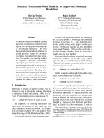
Figure 1: Context reduction and similarity levels
draw this inference, two levels of similarity need to
be taken into account. One concerns the similarity of
the words to be recognised as metonymic or literal
(Possibly Metonymic Words, PMWs). In the above
examples, the PMWs are “Pakistan”, “England” and
“Scotland”. The other level pertains to the similar-
ity between the PMW’s contexts (“<subject> (had)
won the World Cup” and “<subject> lost in the
semi-final”). In this paper, we show how a machine
learning algorithm can exploit both similarities.
Our corpus study on the semantic class of lo-
cations confirms that regular metonymic patterns,
e.g., using a place name for any of its sports teams,
cover most metonymies, whereas unconventional
metonymies like (1) are very rare (Section 2). Thus,
we can recast metonymy resolution as a classifica-
tion task operating on semantic classes (Section 3).
In Section 4, we restrict the classifier’s features to
head-modifier relations involving the PMW. In both
(2) and (3), the context is reduced to subj-of-win.
This allows the inference from (2) to (3), as they
have the same feature value. Although the remain-
ing context is discarded, this feature achieves high
precision. In Section 5, we generalize context simi-
larity to draw inferences from (2) or (3) to (4). We
exploit both the similarity of the heads in the gram-
matical relation (e.g., “win” and “lose”) and that of

the grammatical role (e.g. subject). Figure 1 illus-
trates context reduction and similarity levels.
We evaluate the impact of automatic extraction of
head-modifier relations in Section 6. Finally, we dis-
cuss related work and our contributions.
2 Corpus Study
We summarize (Markert and Nissim, 2002b)’s an-
notation scheme for location names and present an
annotated corpus of occurrences of country names.
2.1 Annotation Scheme for Location Names
We identify literal, metonymic,andmixed readings.
The literal reading comprises a locative (5)
and a political entity interpretation (6).
(5) coral coast of Papua New Guinea
(6) Britain’s current account deficit
We distinguish the following metonymic patterns
(see also (Lakoff and Johnson, 1980; Fass, 1997;
Stern, 1931)). In a place-for-people pattern,
a place stands for any persons/organisations associ-
ated with it, e.g., for sports teams in (2), (3), and (4),
and for the government in (7).
4
(7) a cardinal element in Iran’s strategy when
Iranian naval craft [ ] bombarded [ ]
In a place-for-event pattern, a location
name refers to an event that occurred there (e.g., us-
ing the word Vietnam for the Vietnam war). In a
place-for-product pattern a place stands for
a product manufactured there (e.g., the word Bor-
deaux referring to the local wine).

The category othermet covers unconventional
metonymies, as (1), and is only used if none of the
other categories fits (Markert and Nissim, 2002b).
We also found examples where two predicates are
involved, each triggering a different reading.
(8) they arrived in Nigeria, hitherto a leading
critic of the South African regime
In (8), both a literal (triggered by “arriving in”)
and a place-for-people reading (triggered by
“leading critic”) are invoked. We introduced the cat-
egory mixed to deal with these cases.
2.2 Annotation Results
Using Gsearch (Corley et al., 2001), we randomly
extracted 1000 occurrences of country names from
the BNC, allowing any country name and its variants
listed in the CIA factbook
5
or WordNet (Fellbaum,
4
As the explicit referent is often underspecified, we intro-
duce place-for-people as a supertype category and we
evaluate our system on supertype classification in this paper. In
the annotation, we further specify the different groups of people
referred to, whenever possible (Markert and Nissim, 2002b).
5
/>factbook/
1998) to occur. Each country name is surrounded by
three sentences of context.
The 1000 examples of our corpus have been inde-
pendently annotated by two computational linguists,

who are the authors of this paper. The annotation
can be considered reliable (Krippendorff, 1980) with
95% agreement and a kappa (Carletta, 1996) of .88.
Our corpus for testing and training the algorithm
includes only the examples which both annotators
could agree on and which were not marked as noise
(e.g. homonyms, as “Professor Greenland”), for a
total of 925. Table 1 reports the reading distribution.
Table 1: Distribution of readings in our corpus
reading freq %
literal 737 79.7
place-for-people 161 17.4
place-for-event 3.3
place-for-product 0.0
mixed 15 1.6
othermet 91.0
total non-literal 188 20.3
total 925 100.0
3 Metonymy Resolution as a Classification
Task
The corpus distribution confirms that metonymies
that do not follow established metonymic patterns
(othermet) are very rare. This seems to be the
case for other kinds of metonymies, too (Verspoor,
1997). We can therefore reformulate metonymy res-
olution as a classification task between the literal
reading and a fixed set of metonymic patterns that
can be identified in advance for particular semantic
classes. This approach makes the task comparable to
classic word sense disambiguation (WSD), which is

also concerned with distinguishing between possible
word senses/interpretations.
However, whereas a classic (supervised) WSD
algorithm is trained on a set of labelled instances
of one particular word and assigns word senses to
new test instances of the same word, (supervised)
metonymy recognition can be trained on a set of
labelled instances of different words of one seman-
tic class and assign literal readings and metonymic
patterns to new test instances of possibly different
words of the same semantic class. This class-based
approach enables one to, for example, infer the read-
ing of (3) from that of (2).
We use a decision list (DL) classifier. All features
encountered in the training data are ranked in the DL
(best evidence first) according to the following log-
likelihood ratio (Yarowsky, 1995):
Log

Pr(reading
i
|feature
k
)

j=i
Pr(reading
j
|feature
k

)

We estimated probabilities via maximum likeli-
hood, adopting a simple smoothing method (Mar-
tinez and Agirre, 2000): 0.1 is added to both the de-
nominator and numerator.
The target readings to be distinguished are
literal, place-for-people, place-for-
event, place-for-product, othermet and
mixed. All our algorithms are tested on our an-
notated corpus, employing 10-fold cross-validation.
We evaluate accuracy and coverage:
Acc =
# correct decisions made
# decisions made
Cov =
# decisions made
# test data
We also use a backing-off strategy to the most fre-
quent reading (literal) for the cases where no
decision can be made. We report the results as ac-
curacy backoff (Acc
b
); coverage backoff is always
1. We are also interested in the algorithm’s perfor-
mance in recognising non-literal readings. There-
fore, we compute precision (P ), recall (R), and F-
measure (F ), where A is the number of non-literal
readings correctly identified as non-literal (true pos-
itives) and B the number of literal readings that are

incorrectly identified as non-literal (false positives):
P = A/(A + B)
R =
A
#non-literal examples in the test data
F =2PR/(R + P )
The baseline used for comparison is the assign-
ment of the most frequent reading literal.
4 Context Reduction
We show that reducing the context to head-modifier
relations involving the Possibly Metonymic Word
achieves high precision metonymy recognition.
6
6
In (Markert and Nissim, 2002a), we also considered local
and topical cooccurrences as contextual features. They con-
stantly achieved lower precision than grammatical features.
Table 2: Example feature values for role-of-head
role-of-head (r-of-h) example
subj-of-win England won the World Cup (place-for-people)
subjp-of-govern
Britain has been governed by (literal)
dobj-of-visit
the Apostle had visited Spain (literal)
gen-of-strategy
in Iran’sstrategy (place-for-people)
premod-of-veteran
a Vietnam veteran from Rhode Island (place-for-event)
ppmod-of-with
its border with Hungary (literal)

Table 3: Role distribution
role freq #non-lit
subj 92 65
subjp 64
dobj 28 12
gen 93 20
premod 94 13
ppmod 522 57
other 90 17
total 925 188
We represent each example in our corpus by a sin-
gle feature role-of-head, expressing the grammat-
ical role of the PMW (limited to (active) subject,
passive subject, direct object, modifier in a prenom-
inal genitive, other nominal premodifier, dependent
in a prepositional phrase) and its lemmatised lexi-
cal head within a dependency grammar framework.
7
Table 2 shows example values and Table 3 the role
distribution in our corpus.
We trained and tested our algorithm with this fea-
ture (hmr).
8
Results for hmr are reported in the
first line of Table 5. The reasonably high precision
(74.5%) and accuracy (90.2%) indicate that reduc-
ing the context to a head-modifier feature does not
cause loss of crucial information in most cases. Low
recall is mainly due to low coverage (see Problem 2
below). We identified two main problems.

Problem 1. The feature can be too simplistic, so
that decisions based on the head-modifier relation
can assign the wrong reading in the following cases:
• “Bad” heads: Some lexical heads are semanti-
cally empty, thus failing to provide strong evi-
dence for any reading and lowering both recall
and precision. Bad predictors are the verbs “to
have” and “to be” and some prepositions such
as “with”, which can be used with metonymic
(talk with Hungary) and literal (border with
Hungary) readings. This problem is more se-
rious for function than for content word heads:
precision on the set of subjects and objects is
81.8%, but only 73.3% on PPs.
• “Bad” relations: The premod relation suffers
from noun-noun compound ambiguity. US op-
7
We consider only one link per PMW, although cases like (8)
would benefit from including all links the PMW participates in.
8
The feature values were manually annotated for the follow-
ing experiments, adapting the guidelines in (Poesio, 2000). The
effect of automatic feature extraction is described in Section 6.
eration can refer to an operation in the US (lit-
eral) or by the US (metonymic).
• Other cases: Very rarely neglecting the remain-
ing context leads to errors, even for “good”
lexical heads and relations. Inferring from the
metonymy in (4) that “Germany” in “Germany
lost a fifth of its territory” is also metonymic,

e.g., is wrong and lowers precision.
However, wrong assignments (based on head-
modifier relations) do not constitute a major problem
as accuracy is very high (90.2%).
Problem 2. The algorithm is often unable to make
any decision that is based on the head-modifier re-
lation. This is by far the more frequent problem,
which we adress in the remainder of the paper. The
feature role-of-head accounts for the similarity be-
tween (2) and (3) only, as classification of a test in-
stance with a particular feature value relies on hav-
ing seen exactly the same feature value in the train-
ing data. Therefore, we have not tackled the infer-
ence from (2) or (3) to (4). This problem manifests
itself in data sparseness and low recall and coverage,
as many heads are encountered only once in the cor-
pus. As hmr’s coverage is only 63.1%, backoff to a
literal reading is required in 36.9% of the cases.
5 Generalising Context Similarity
In order to draw the more complex inference from
(2) or (3) to (4) we need to generalise context sim-
ilarity. We relax the identity constraint of the orig-
inal algorithm (the same role-of-head value of the
test instance must be found in the DL), exploiting
two similarity levels. Firstly, we allow to draw infer-
ences over similar values of lexical heads (e.g. from
subj-of-win to subj-of-lose), rather than over iden-
tical ones only. Secondly, we allow to discard the
Table 4: Example thesaurus entries
lose[V]: win

1
0.216,gain
2
0.209, have
3
0.207,
attitude[N]:stance
1
0.181, behavior
2
0.18, , strategy
17
0.128
lexical head and generalise over the PMW’s gram-
matical role (e.g. subject). These generalisations al-
low us to double recall without sacrificing precision
or increasing the size of the training set.
5.1 Relaxing Lexical Heads
We regard two feature values r-of-h and r-of-h

as
similar if h and h

are similar. In order to capture the
similarity between h and h

we integrate a thesaurus
(Lin, 1998) in our algorithm’s testing phase. In Lin’s
thesaurus, similarity between words is determined
by their distribution in dependency relations in a

newswire corpus. For a content word h (e.g., “lose”)
of a specific part-of-speech a set of similar words Σ
h
of the same part-of-speech is given. The set mem-
bers are ranked in decreasing order by a similarity
score. Table 4 reports example entries.
9
Our modified algorithm (relax I) is as follows:
1. train DL with role-of-head as in hmr; for each test in-
stance observe the following procedure (r-of-h indicates
the feature value of the test instance);
2. if r-of-h is found in the DL, apply the corresponding rule
and stop;
2

otherwise choose a number n ≥ 1 and set i =1;
(a) extract the i
th
most similar word h
i
to h from the
thesaurus;
(b) if i>nor the similarity score of h
i
< 0.10, assign
no reading and stop;
(b’) otherwise:ifr-of-h
i
is found in the DL, apply cor-
responding rule and stop; if r-of-h

i
is not found in
the DL, increase i by 1 and go to (a);
The examples already covered by hmr are clas-
sified in exactly the same way by relax I (see Step
2). Let us therefore assume we encounter the test
instance (4), its feature value subj-of-lose has not
been seen in the training data (so that Step 2 fails
and Step 2

has to be applied) and subj-of-win is in
the DL. For all n ≥ 1, relax I will use the rule for
subj-of-win to assign a reading to “Scotland” in (4)
as “win” is the most similar word to “lose” in the
thesaurus (see Table 4). In this case (2b’) is only
9
In the original thesaurus, each Σ
h
is subdivided into clus-
ters. We do not take these divisions into account.
0 10203040
50
Thesaurus Iterations (n)
0.1 0.1
0.2 0.2
0.3 0.3
0.4 0.4
0.5 0.5
0.6 0.6
0.7 0.7

0.8 0.8
0.9 0.9
Results
Precision
Recall
F-Measure
Figure 2: Results for relax I
applied once as already the first iteration over the
thesaurus finds a word h
1
with r-of-h
1
in the DL.
The classification of “Turkey” with feature value
gen-of-attitude in (9) required 17 iterations to find
awordh
17
(“strategy”; see Example (7)) similar to
“attitude”, with r-of-h
17
(gen-of-strategy)intheDL.
(9) To say that this sums up Turkey’s attitude as
a whole would nevertheless be untrue
Precision, recall and F-measure for n ∈
{1, , 10, 15, 20, 25, 30, 40, 50} are visualised in
Figure 2. Both precision and recall increase with
n. Recall more than doubles from 18.6% in hmr
to 41% and precision increases from 74.5% in hmr
to 80.2%, yielding an increase in F-measure from
29.8% to 54.2% (n =50). Coverage rises to 78.9%

and accuracy backoff to 85.1% (Table 5).
Whereas the increase in coverage and recall is
quite intuitive, the high precision achieved by re-
lax I requires further explanation. Let S be the set
of examples that relax I covers. It consists of two
subsets: S1 is the subset already covered by hmr and
its treatment does not change in relax I, yielding the
same precision. S2 is the set of examples that re-
lax I covers in addition to hmr. The examples in S2
consist of cases with highly predictive content word
heads as (a) function words are not included in the
thesaurus and (b) unpredictive content word heads
like “have” or “be” are very frequent and normally
already covered by hmr (they are therefore members
of S1). Precision on S2 is very high (84%) and raises
the overall precision on the set S.
Cases that relax I does not cover are mainly due
to (a) missing thesaurus entries (e.g., many proper
Table 5: Results summary for manual annotation.
For relax I and combination we report best results
(50 thesaurus iterations).
algorithm Acc Cov Acc
b
PRF
hmr .902 .631 .817 .745 .186 .298
relax I .877 .789 .851 .802 .410 .542
relax II
.865 .903 .859 .813 .441 .572
combination .894 .797 .870 .814 .510 .627
baseline .797 1.00 .797 n/a .000 n/a

names or alternative spelling), (b) the small num-
ber of training instances for some grammatical roles
(e.g. dobj), so that even after 50 thesaurus iterations
no similar role-of-head value could be found that is
covered in the DL, or (c) grammatical roles that are
not covered (other in Table 3).
5.2 Discarding Lexical Heads
Another way of capturing the similarity between (3)
and (4), or (7) and (9) is to ignore lexical heads and
generalise over the grammatical role (role)ofthe
PMW (with the feature values as in Table 3: subj,
subjp, dobj, gen, premod, ppmod). We therefore de-
veloped the algorithm relax II.
1. train decision lists:
(a) DL1 with role-of-head as in hmr
(b) DL2 with role;
for each test instance observe the following procedure (r-
of-h and r are the feature values of the test instance);
2. if r-of-h is found in the DL1, apply the corresponding rule
and stop;
2’ otherwise,ifr is found in DL2, apply the corresponding
rule.
Let us assume we encounter the test instance
(4), subj-of-lose is not in DL1 (so that Step 2 fails
and Step 2

has to be applied) and subj is in DL2.
The algorithm relax II will assign a place-for-
people reading to “Scotland”, as most subjects in
our corpus are metonymic (see Table 3).

Generalising over the grammatical role outper-
forms hmr, achieving 81.3% precision, 44.1% re-
call, and 57.2% F-measure (see Table 5). The algo-
rithm relax II also yields fewer false negatives than
relax I (and therefore higher recall) since all sub-
jects not covered in DL1 are assigned a metonymic
reading, which is not true for relax I.
5.3 Combining Generalisations
There are several ways of combining the algorithms
we introduced. In our experiments, the most suc-
cessful one exploits the facts that relax II performs
better than relax I on subjects and that relax I per-
forms better on the other roles. Therefore the algo-
rithm combination uses relax II if the test instance
is a subject, and relax I otherwise. This yields the
best results so far, with 87% accuracy backoff and
62.7% F-measure (Table 5).
6 Influence of Parsing
The results obtained by training and testing our clas-
sifier with manually annotated grammatical relations
are the upper bound of what can be achieved by us-
ing these features. To evaluate the influence pars-
ing has on the results, we used the RASP toolkit
(Briscoe and Carroll, 2002) that includes a pipeline
of tokenisation, tagging and state-of-the-art statisti-
cal parsing, allowing multiple word tags. The toolkit
also maps parse trees to representations of gram-
matical relations, which we in turn could map in a
straightforward way to our role categories.
RASP produces at least partial parses for 96% of

our examples. However, some of these parses do
not assign any role of our roleset to the PMW —
only 76.9% of the PMWs are assigned such a role
by RASP (in contrast to 90.2% in the manual anno-
tation; see Table 3). RASP recognises PMW sub-
jects with 79% precision and 81% recall. For PMW
direct objects, precision is 60% and recall 86%.
10
We reproduced all experiments using the auto-
matically extracted relations. Although the relative
performance of the algorithms remains mostly un-
changed, most of the resulting F-measures are more
than 10% lower than for hand annotated roles (Ta-
ble 6). This is in line with results in (Gildea and
Palmer, 2002), who compare the effect of man-
ual and automatic parsing on semantic predicate-
argument recognition.
7 Related Work
Previous Approaches to Metonymy Recognition.
Our approach is the first machine learning algorithm
to metonymy recognition, building on our previous
10
We did not evaluate RASP’s performance on relations that
do not involve the PMW.
Table 6: Results summary for the different algo-
rithms using RASP. For relax I and combination
we report best results (50 thesaurus iterations).
algorithm Acc Cov Acc
b
PRF

hmr .884 .514 .812 .674 .154 .251
relax I .841 .666 .821 .619 .319 .421
relax II
.820 .769 .823 .621 .340 .439
combination .850 .672 .830 .640 .388 .483
baseline .797 1.00 .797 n/a .000 n/a
work (Markert and Nissim, 2002a). The current ap-
proach expands on it by including a larger number
of grammatical relations, thesaurus integration, and
an assessment of the influence of parsing. Best F-
measure for manual annotated roles increased from
46.7% to 62.7% on the same dataset.
Most other traditional approaches rely on hand-
crafted knowledge bases or lexica and use vi-
olations of hand-modelled selectional restrictions
(plus sometimes syntactic violations) for metonymy
recognition (Pustejovsky, 1995; Hobbs et al., 1993;
Fass, 1997; Copestake and Briscoe, 1995; Stallard,
1993).
11
In these approaches, selectional restric-
tions (SRs) are not seen as preferences but as ab-
solute constraints. If and only if such an absolute
constraint is violated, a non-literal reading is pro-
posed. Our system, instead, does not have any a
priori knowledge of semantic predicate-argument re-
strictions. Rather, it refers to previously seen train-
ing examples in head-modifier relations and their la-
belled senses and computes the likelihood of each
sense using this distribution. This is an advantage as

our algorithm also resolved metonymies without SR
violations in our experiments. An empirical compar-
ison between our approach in (Markert and Nissim,
2002a)
12
and an SRs violation approach showed that
our approach performed better.
In contrast to previous approaches (Fass, 1997;
Hobbs et al., 1993; Copestake and Briscoe, 1995;
Pustejovsky, 1995; Verspoor, 1996; Markert and
Hahn, 2002; Harabagiu, 1998; Stallard, 1993), we
use a corpus reliably annotated for metonymy for
evaluation, moving the field towards more objective
11
(Markert and Hahn, 2002) and (Harabagiu, 1998) en-
hance this with anaphoric information. (Briscoe and Copes-
take, 1999) propose using frequency information besides syn-
tactic/semantic restrictions, but use only a priori sense frequen-
cies without contextual features.
12
Note that our current approach even outperforms (Markert
and Nissim, 2002a).
evaluation procedures.
Word Sense Disambiguation. We compared our
approach to supervised WSD in Section 3, stressing
word-to-word vs. class-to-class inference. This al-
lows for a level of abstraction not present in standard
supervised WSD. We can infer readings for words
that have not been seen in the training data before,
allow an easy treatment of rare words that undergo

regular sense alternations and do not have to anno-
tate and train separately for every individual word to
treat regular sense distinctions.
13
By exploiting additional similarity levels and inte-
grating a thesaurus we further generalise the kind of
inferences we can make and limit the size of anno-
tated training data: as our sampling frame contains
553 different names, an annotated data set of 925
samples is quite small. These generalisations over
context and collocates are also applicable to stan-
dard WSD and can supplement those achieved e.g.,
by subcategorisation frames (Martinez et al., 2002).
Our approach to word similarity to overcome data
sparseness is perhaps most similar to (Karov and
Edelman, 1998). However, they mainly focus on the
computation of similarity measures from the train-
ing data. We instead use an off-the-shelf resource
without adding much computational complexity and
achieve a considerable improvement in our results.
8 Conclusions
We presented a supervised classification algorithm
for metonymy recognition, which exploits the simi-
larity between examples of conventional metonymy,
operates on semantic classes and thereby enables
complex inferences from training to test examples.
We showed that syntactic head-modifier relations
are a high precision feature for metonymy recogni-
tion. However, basing inferences only on the lex-
ical heads seen in the training data leads to data

sparseness due to the large number of different lex-
ical heads encountered in natural language texts. In
order to overcome this problem we have integrated
a thesaurus that allows us to draw inferences be-
13
Incorporating knowledge about particular PMWs (e.g., as
a prior) will probably improve performance, as word idiosyn-
cracies — which can still exist even when treating regular sense
distinctions — could be accounted for. In addition, knowledge
about the individual word is necessary to assign its original se-
mantic class.
tween examples with similar but not identical lex-
ical heads. We also explored the use of simpler
grammatical role features that allow further gener-
alisations. The results show a substantial increase in
precision, recall and F-measure. In the future, we
will experiment with combining grammatical fea-
tures and local/topical cooccurrences. The use of
semantic classes and lexical head similarity gener-
alises over two levels of contextual similarity, which
exceeds the complexity of inferences undertaken in
standard supervised word sense disambiguation.
Acknowledgements. The research reported in this
paper was supported by ESRC Grant R000239444.
Katja Markert is funded by an Emmy Noether Fel-
lowship of the Deutsche Forschungsgemeinschaft
(DFG). We thank three anonymous reviewers for
their comments and suggestions.
References
E. Briscoe and J. Carroll. 2002. Robust accurate statisti-

cal annotation of general text. In Proc. of LREC, 2002,
pages 1499–1504.
T. Briscoe and A. Copestake. 1999. Lexical rules in
constraint-based grammar. Computational Linguis-
tics, 25(4):487–526.
J. Carletta. 1996. Assessing agreement on classification
tasks: The kappa statistic. Computational Linguistics,
22(2):249–254.
A. Copestake and T. Briscoe. 1995. Semi-productive
polysemy and sense extension. Journal of Semantics,
12:15–67.
S. Corley, M. Corley, F. Keller, M. Crocker, and S.
Trewin. 2001. Finding syntactic structure in unparsed
corpora: The Gsearch corpus query system. Comput-
ers and the Humanities, 35(2):81–94.
D. Fass. 1997. Processing Metaphor and Metonymy.
Ablex, Stanford, CA.
C. Fellbaum, ed. 1998. WordNet: An Electronic Lexical
Database. MIT Press, Cambridge, Mass.
D. Gildea and M. Palmer. 2002. The necessity of parsing
for predicate argument recognition. In Proc. of ACL,
2002, pages 239–246.
S. Harabagiu. 1998. Deriving metonymic coercions
from WordNet. In Workshop on the Usage of WordNet
in Natural Language Processing Systems, COLING-
ACL, 1998, pages 142–148.
J. R. Hobbs, M. E. Stickel, D. E. Appelt, and P. Martin.
1993. Interpretation as abduction. Artificial Intelli-
gence, 63:69–142.
S. Kamei and T. Wakao. 1992. Metonymy: Reassess-

ment, survey of acceptability and its treatment in ma-
chine translation systems. In Proc. of ACL, 1992,
pages 309–311.
Y. Karov and S. Edelman. 1998. Similarity-based
word sense disambiguation. Computational Linguis-
tics, 24(1):41-59.
K. Krippendorff. 1980. Content Analysis: An Introduc-
tion to Its Methodology. Sage Publications.
G. Lakoff and M. Johnson. 1980. Metaphors We Live By.
Chicago University Press, Chicago, Ill.
D. Lin. 1998. An information-theoretic definition of
similarity. In Proc. of International Conference on
Machine Learning, Madison, Wisconsin.
K. Markert and U. Hahn. 2002. Understanding
metonymies in discourse. Artificial Intelligence,
135(1/2):145–198.
K. Markert and M. Nissim. 2002a. Metonymy resolu-
tion as a classification task. In Proc. of EMNLP, 2002,
pages 204–213.
Katja Markert and Malvina Nissim. 2002b. Towards a
corpus annotated for metonymies: the case of location
names. In Proc. of LREC, 2002, pages 1385–1392.
D. Martinez and E. Agirre. 2000. One sense per collo-
cation and genre/topic variations. In Proc. of EMNLP,
2000.
D. Martinez, E. Agirre, and L. Marquez. 2002. Syntactic
features for high precision word sense disambiguation.
In Proc. of COLING, 2002.
G. Nunberg. 1978. The Pragmatics of Reference.Ph.D.
thesis, City University of New York, New York.

G. Nunberg. 1995. Transfers of meaning. Journal of
Semantics, 12:109–132.
M. Poesio, 2000. The GNOME Annotation Scheme Man-
ual. University of Edinburgh, 4
th
version. Available
from />J. Pustejovsky. 1995. The Generative Lexicon.MIT
Press, Cambridge, Mass.
D. Stallard. 1993. Two kinds of metonymy. In Proc. of
ACL, 1993, pages 87–94.
G. Stern. 1931. Meaning and Change of Meaning.
G¨oteborg: Wettergren & Kerbers F¨orlag.
C. Verspoor. 1996. Lexical limits on the influence of
context. In Proc. of CogSci, 1996, pages 116–120.
C. Verspoor. 1997. Conventionality-governed logical
metonymy. In H. Bunt et al., editors, Proc. of IWCS-2,
1997, pages 300–312.
D. Yarowsky. 1995. Unsupervised word sense disam-
biguation rivaling supervised methods. In Proc. of
ACL, 1995, pages 189–196.