Tài liệu Báo cáo khoa học: "Fast Decoding and Optimal Decoding for Machine Translation" doc

Fast Decoding and Optimal Decoding for Machine Translation
Ulrich Germann , Michael Jahr , Kevin Knight , Daniel Marcu , and Kenji Yamada
Information Sciences Institute Department of Computer Science
University of Southern California Stanford University
4676 Admiralty Way, Suite 1001 Stanford, CA 94305
Marina del Rey, CA 90292
germann,knight,marcu,kyamada @isi.edu
Abstract
A good decoding algorithm is critical
to the success of any statistical machine
translation system. The decoder’s job is
to find the translation that is most likely
according to set of previously learned
parameters (and a formula for combin-
ing them). Since the space of possi-
ble translations is extremely large, typ-
ical decoding algorithms are only able
to examine a portion of it, thus risk-
ing to miss good solutions. In this pa-
per, we compare the speed and out-
put quality of a traditional stack-based
decoding algorithm with two new de-
coders: a fast greedy decoder and a
slow but optimal decoder that treats de-
coding as an integer-programming opti-
mization problem.
1 Introduction
A statistical MT system that translates (say)
French sentences into English, is divided into
three parts: (1) a language model (LM) that as-
signs a probability P(e) toany English string, (2) a

translation model (TM) that assigns a probability
P(f
e) to any pair of English and French strings,
and (3) a decoder. The decoder takes a previ-
ously unseen sentence and tries to find the
that maximizes P(e f), or equivalently maximizes
P(e) P(f e).
Brown et al. (1993) introduced a series of
TMs based on word-for-word substitution and re-
ordering, but did not include a decoding algo-
rithm. If the source and target languages are con-
strained to have the same word order (by choice
or through suitable pre-processing), then the lin-
ear Viterbi algorithm can be applied (Tillmann et
al., 1997). If re-ordering is limited to rotations
around nodes in a binary tree, then optimal decod-
ing can be carried out by a high-polynomial algo-
rithm (Wu, 1996). For arbitrary word-reordering,
the decoding problem is NP-complete (Knight,
1999).
A sensible strategy (Brown et al., 1995; Wang
and Waibel, 1997) is to examine a large subset of
likely decodings and choose just from that. Of
course, it is possible to miss a good translation
this way. If the decoder returns e
but there exists
some e for which P(e f) P(e f), this is called
a search error. As Wang and Waibel (1997) re-
mark, it is hard to know whether a search error
has occurred—the only way to show that a decod-

ing is sub-optimal is to actually produce a higher-
scoring one.
Thus, while decoding is a clear-cut optimiza-
tion task in which every problem instance has a
right answer, it is hard to come up with good
answers quickly. This paper reports on mea-
surements of speed, search errors, and translation
quality in the context of a traditional stack de-
coder (Jelinek, 1969; Brown et al., 1995) and two
new decoders. The first is a fast greedy decoder,
and the second is a slow optimal decoder based on
generic mathematical programming techniques.
2 IBM Model 4
In this paper, we work with IBM Model 4, which
revolves around the notion of a word alignment
over a pair of sentences (see Figure 1). A word
alignment assigns a single home (English string
position) to each French word. If two French
words align to the same English word, then that
it is not clear .
| \ | \ \
| \ + \ \
| \/ \ \ \
| /\ \ \ \
CE NE EST PAS CLAIR .
Figure 1: Sample word alignment.
English word is said to have a fertility of two.
Likewise, if an English word remains unaligned-
to, then it has fertility zero. The word align-
ment in Figure 1 is shorthand for a hypothetical

stochastic process by which an English string gets
converted into a French string. There are several
sets of decisions to be made.
First, every English word is assigned a fertil-
ity. These assignments are made stochastically
according to a table n(
e ). We delete from
the string any word with fertility zero, we dupli-
cate any word with fertility two, etc. If a word has
fertility greater than zero, we call it fertile. If its
fertility is greater than one, we call it very fertile.
After each English word in the new string, we
may increment the fertility of an invisible En-
glish NULL element with probability p
(typi-
cally about 0.02). The NULL element ultimately
produces “spurious” French words.
Next, we perform a word-for-word replace-
ment of English words (including NULL) by
French words, according to the table t(f e ).
Finally, we permute the French words. In per-
muting, Model 4 distinguishes between French
words that are heads (the leftmost French word
generated from a particular English word), non-
heads (non-leftmost, generated only by very fer-
tile English words), and NULL-generated.
Heads. The head of one English word is as-
signed a French string position based on the po-
sition assigned to the previous English word. If
an English word e

translates into something
at French position j, then the French head word
of e is stochastically placed in French position
k with distortion probability d (k–j class(e ),
class(f )), where “class” refers to automatically
determined word classes for French and English
vocabulary items. This relative offset k–j encour-
ages adjacent English words to translate into ad-
jacent French words. If e is infertile, then j is
taken from e , etc. If e is very fertile, then j
is the average of the positions of its French trans-
lations.
Non-heads. If the head of English word e
is placed in French position j, then its first non-
head is placed in French position k ( j) accord-
ing to another table d (k–j class(f )). The next
non-head is placed at position q with probability
d
(q–k class(f )), and so forth.
NULL-generated. After heads and non-heads
are placed, NULL-generated words are permuted
into the remaining vacant slots randomly. If there
are NULL-generated words, then any place-
ment scheme is chosen with probability 1/ .
These stochastic decisions, starting with e, re-
sult in different choices of f and an alignment of f
with e. We map an e onto a particular
a,f pair
with probability:
P(a, f e) =

n e t e
d e
d
NULL
where the factors separated by symbols denote
fertility, translation, head permutation, non-head
permutation, null-fertility, and null-translation
probabilities.
1
3 Definition of the Problem
If we observe a new sentence f, then an optimal
decoder will search for an e that maximizes P(e
f)
1
The symbols in this formula are: (the length of e),
(the length off), e (the i English word in e), e (the NULL
word),
(the fertility of e ), (the fertility of the NULL
word), (the k French word produced by e in a),
(the position of in f), (the position of the first fertile
word to the left of e in a), (the ceiling of the average of
all for , or 0 if is undefined).
P(e) P(f e). Here, P(f e) is the sum of P(a,f e)
over all possible alignments a. Because this
sum involves significant computation, we typi-
cally avoid it by instead searching for an e,a
pair that maximizes P(e,a f) P(e) P(a,f e). We
take the language model P(e) to be a smoothed
n-gram model of English.
4 Stack-Based Decoding

The stack (also called A*) decoding algorithm is
a kind of best-first search which was first intro-
duced in the domain of speech recognition (Je-
linek, 1969). By building solutions incremen-
tally and storing partial solutions, or hypotheses,
in a “stack” (in modern terminology, a priority
queue), the decoder conducts an ordered search
of the solution space. In the ideal case (unlimited
stack size and exhaustive search time), a stack de-
coder is guaranteed to find an optimal solution;
our hope is to do almost as well under real-world
constraints of limited space and time. The generic
stack decoding algorithm follows:
Initialize the stack with an empty hy-
pothesis.
Pop h, the best hypothesis, off the stack.
If h is a complete sentence, output h and
terminate.
For each possible next word w, extend h
by adding w and push the resulting hy-
pothesis onto the stack.
Return to the second step (pop).
One crucial difference between the decoding
process in speech recognition (SR) and machine
translation (MT) is that speech is always pro-
duced in the same order as its transcription. Con-
sequently, in SR decoding there is always a sim-
ple left-to-right correspondence between input
and output sequences. By contrast, in MT the left-
to-right relation rarely holds even for language

pairs as similar as French and English. We ad-
dress this problem by building the solution from
left to right, but allowing the decoder to consume
its input in any order. This change makes decod-
ing significantly more complex in MT; instead of
knowing the order of the input in advance, we
must consider all
permutations of an -word
input sentence.
Another important difference between SR and
MT decoding is the lack of reliable heuristics
in MT. A heuristic is used in A* search to es-
timate the cost of completing a partial hypothe-
sis. A good heuristic makes it possible to accu-
rately compare the value of different partial hy-
potheses, and thus to focus the search in the most
promising direction. The left-to-right restriction
in SR makes it possible to use a simple yet reli-
able class of heuristics which estimate cost based
on the amount of input left to decode. Partly be-
cause of the absence of left-to-right correspon-
dence, MT heuristics are significantly more dif-
ficult to develop (Wang and Waibel, 1997). With-
out a heuristic, a classic stack decoder is inef-
fective because shorter hypotheses will almost al-
ways look more attractive than longer ones, since
as we add words to a hypothesis, we end up mul-
tiplying more and more terms to find the proba-
bility. Because of this, longer hypotheses will be
pushed off the end of the stack by shorter ones

even if they are in reality better decodings. For-
tunately, by using more than one stack, we can
eliminate this effect.
In a multistack decoder, we employ more than
one stack to force hypotheses to compete fairly.
More specifically, we have one stack for each sub-
set of input words. This way, a hypothesis can
only be pruned if there are other, better, hypothe-
ses that represent the same portion of the input.
With more than one stack, however, how does a
multistack decoder choose which hypothesis to
extend during each iteration? We address this is-
sue by simply taking one hypothesis from each
stack, but a better solution would be to somehow
compare hypotheses from different stacks and ex-
tend only the best ones.
The multistack decoder we describe is closely
patterned on the Model 3 decoder described in the
(Brown et al., 1995) patent. We build solutions
incrementally by applying operations to hypothe-
ses. There are four operations:
Add adds a new English word and
aligns a single French word to it.
AddZfert adds two new English words.
The first has fertility zero, while the
second is aligned to a single French
word.
Extend aligns an additional French
word to the most recent English word,
increasing its fertility.

AddNull aligns a French word to the
English NULL element.
AddZfert is by far the most expensive opera-
tion, as we must consider inserting a zero-fertility
English word before each translation of each un-
aligned French word. With an English vocabulary
size of 40,000, AddZfert is 400,000 times more
expensive than AddNull!
We can reduce the cost of AddZfert in two
ways. First, we can consider only certain English
words as candidates for zero-fertility, namely
words which both occur frequently and have
a high probability of being assigned frequency
zero. Second, we can only insert a zero-fertility
word if it will increase theprobability of a hypoth-
esis. According to the definition of the decoding
problem, a zero-fertility English word can only
make a decoding more likely by increasing P(e)
more than it decreases P(a,f
e).
2
By only con-
sidering helpful zero-fertility insertions, we save
ourselves significant overhead in the AddZfert
operation, in many cases eliminating all possi-
bilities and reducing its cost to less than that of
AddNull.
5 Greedy Decoding
Over the last decade, many instances of NP-
complete problems have been shown to be solv-

able in reasonable/polynomial time using greedy
methods (Selman et al., 1992; Monasson et al.,
1999). Instead of deeply probing the search
space, such greedy methods typically start out
with a random, approximate solution and then try
to improve it incrementally until a satisfactory so-
lution is reached. In many cases, greedy methods
quickly yield surprisingly good solutions.
We conjectured that such greedy methods may
prove to be helpful in the context of MT decod-
ing. The greedy decoder that we describe starts
the translation process from an English gloss of
the French sentence given as input. The gloss
is constructed by aligning each French word f
with its most likely English translation e
f
(e
f
argmax t(e f )). For example, in translating the
French sentence “Bien entendu , il parle de une
belle victoire .”, the greedy decoder initially as-
2
We know that adding a zero-fertility word will decrease
P(a,f e) because it adds a term n(0 e ) 1 to the calculation.
sumes that a good translation of it is “Well heard
, it talking a beautiful victory” because the best
translation of “bien” is “well”, the best translation
of “entendu” is “heard”, and so on. The alignment
corresponding to this translation is shown at the
top of Figure 2.

Once the initial alignment is created, the
greedy decoder tries to improve it, i.e., tries to
find an alignment (and implicitly translation) of
higher probability, by applying one of the follow-
ing operations:
translateOneOrTwoWords( ,e , ,e )
changes the translation of one or two French
words, those located at positions and ,
from e
and e into e and e . If e is
a word of fertility 1 and e is NULL, then
e is deleted from the translation. If e is
the NULL word, the word e is inserted into
the translation at the position that yields the
alignment of highest probability. If e
e or e e , this operation amounts to
changing the translation of a single word.
translateAndInsert( ,e ,e ) changes the
translation of the French word located at po-
sition from e into and simulataneously
inserts word e at the position that yields the
alignment of highest probability. Word
is selected from an automatically derived list
of 1024 words with high probability of hav-
ing fertility 0. When e e , this operation
amounts to inserting a word of fertility 0 into
the alignment.
removeWordOfFertility0( ) deletes the
word of fertility 0 at position in the current
alignment.

swapSegments( ) creates a new
alignment from the old one by swap-
ping non-overlapping English word seg-
ments and . During the swap
operation, all existing links between English
and French words are preserved. The seg-
ments can be as small as a word or as long as
words, where is the length of
the English sentence.
joinWords( ) eliminates from the align-
ment the English word at position (or )
and links the French words generated by
(or ) to (or ).
Figure 2: Example of how the greedy decoder
produces the translation of French sentence “Bien
entendu, il parle de une belle victoire.”
In a stepwise fashion, starting from the initial
gloss, the greedy decoder iterates exhaustively
over all alignments that are one operation away
from the alignment under consideration. At every
step, the decoder chooses the alignment of high-
est probability, until the probability of the current
alignment can no longer be improved. When it
starts from the gloss of the French sentence “Bien
entendu, il parle de une belle victoire.”, for ex-
ample, the greedy decoder alters the initial align-
ment incrementally as shown in Figure 2, eventu-
ally producing the translation “Quite naturally, he
talks about a great victory.”. In the process, the
decoder explores a total of 77421 distinct align-

ments/translations, of which “Quite naturally, he
talks about a great victory.” has the highest prob-
ability.
We chose the operation types enumerated
above for two reasons: (i) they are general enough
to enable the decoder escape local maxima and
modify in a non-trivial manner a given align-
ment in order to produce good translations; (ii)
they are relatively inexpensive (timewise). The
most time consuming operations in the decoder
are swapSegments, translateOneOrTwoWords,
and translateAndInsert. SwapSegments iter-
ates over all possible non-overlapping span pairs
that can be built on a sequence of length
.
TranslateOneOrTwoWords iterates over
alignments, where is the size of the
French sentence and is the number of trans-
lations we associate with each word (in our im-
plementation, we limit this number to the top 10
translations). TranslateAndInsert iterates over
alignments, where is the
size of the list of words with high probability of
having fertility 0 (1024 words in our implementa-
tion).
6 Integer Programming Decoding
Knight (1999) likens MT decoding to finding
optimal tours in the Traveling Salesman Prob-
lem (Garey and Johnson, 1979)—choosing a
good word order for decoder output is similar

to choosing a good TSP tour. Because any TSP
problem instance can be transformed into a de-
coding problem instance, Model 4 decoding is
provably NP-complete in the length of f. It is
interesting to consider the reverse direction—is
it possible to transform a decoding problem in-
stance into a TSP instance? If so, we may take
great advantage of previous research into efficient
TSP algorithms. We may also take advantage of
existing software packages, obtaining a sophisti-
cated decoder with little programming effort.
It is difficult to convert decoding into straight
TSP, but a wide range of combinatorial optimiza-
tion problems (including TSP) can be expressed
in the more general framework of linear integer
programming. A sample integer program (IP)
looks like this:
minimize objective function:
3.2 * x1 + 4.7 * x2 - 2.1 * x3
subject to constraints:
x1 - 2.6 * x3 > 5
7.3 * x2 > 7
A solution to an IP is an assignment of inte-
ger values to variables. Solutions are constrained
by inequalities involving linear combinations of
variables. An optimal solution is one that re-
spects the constraints and minimizes the value of
the objective function, which is also a linear com-
bination of variables. We can solve IP instances
with generic problem-solving software such as

lp
solve or CPLEX.
3
In this section we explain
3
Available at solve and
.
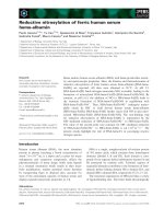
Figure 3: A salesman graph for the input sen-
tence f = “CE NE EST PAS CLAIR .” There is
one city for each word in f. City boundaries are
marked with bold lines, and hotels are illustrated
with rectangles. A tour of cities is a sequence
of hotels (starting at the sentence boundary hotel)
that visits each city exactly once before returning
to the start.
how to express MT decoding (Model 4 plus En-
glish bigrams) in IP format.
We first create a salesman graph like the one
in Figure 3. To do this, we set up a city for each
word in the observed sentence f. City boundaries
are shown with bold lines. We populate each city
with ten hotels corresponding to ten likely En-
glish word translations. Hotels are shown as small
rectangles. The owner of a hotel is the English
word inside the rectangle. If two cities have hotels
with the same owner x, then we build a third x-
owned hotel on the border of the two cities. More
generally, if
cities all have hotels owned by x,
we build new hotels (one for each

non-empty, non-singleton subset of the cities) on
various city borders and intersections. Finally, we
add an extra city representing the sentence bound-
ary.
We define a tour of cities as a sequence and ho-
tels (starting at the sentence boundary hotel) that
visits each city exactly once before returning to
the start. If a hotel sits on the border between two
cities, then staying at that hotel counts as visit-
ing both cities. We can view each tour of cities
as corresponding to a potential decoding e,a .
The owners of the hotels on the tour give us e,
while the hotel locations yield a.
The next task is to establish real-valued (asym-
metric) distances between pairs of hotels, such
that the length of any tour is exactly the negative
of log(P(e)
P(a,f e)). Because log is monotonic,
the shortest tour will correspond to the likeliest
decoding.
The distance we assign to each pair of hotels
consists of some small piece of the Model 4 for-
mula. The usual case is typified by the large black
arrow in Figure 3. Because the destination ho-
tel “not” sits on the border between cities NE
and PAS, it corresponds to a partial alignment in
which the word “not” has fertility two:
what not
/ __/\_
/ / \

CE NE EST PAS CLAIR .
If we assume that we have already paid the
price for visiting the “what” hotel, then our inter-
hotel distance need only account for the partial
alignment concerning “not”:
distance =
– log(bigram(not
what))
– log(n(2
not))
– log(t(NE not)) – log(t(PAS not))
– log(d (+1 class(what), class(NE)))
– log(d (+2 class(PAS)))
NULL-owned hotels are treated specially. We
require that all non-NULL hotels be visited be-
fore any NULL hotels, and we further require that
at most one NULL hotel visited on a tour. More-
over, the NULL fertility sub-formula is easy to
compute if we allow only one NULL hotel to be
visited: is simply the number of cities that ho-
tel straddles, and is the number of cities minus
one. This case is typified by the large gray arrow
shown in Figure 3.
Between hotels that are located (even partially)
in the same city, we assign an infinite distance in
both directions, as travel from one to the other can
never be part of a tour. For 6-word French sen-
tences, we normally come up with a graph that has
about 80 hotels and 3500 finite-cost travel seg-
ments.

The next step is to cast tour selection as an inte-
ger program. Here we adapt a subtour elimination
strategy used in standard TSP. We create a binary
(0/1) integer variable for each pair of hotels
and . if and only if travel from hotel to
hotel is on the itinerary. The objective function
is straightforward:
minimize: distance
This minimization is subject to three classes of
constraints. First, every city must be visited ex-
actly once. That means exactly one tour segment
must exit each city:
located at least
partially in
Second, the segments must be linked to one
another, i.e., every hotel has either (a) one tour
segment coming in and one going out, or (b) no
segments in and none out. To put it another way,
every hotel must have an equal number of tour
segments going in and out:
Third, it is necessary to prevent multiple inde-
pendent sub-tours. To do this, we require that ev-
ery proper subset of cities have at least one tour
segment leaving it:
located
entirely
within
located
at least
partially

outside
There are an exponential number of constraints in
this third class.
Finally, we invoke our IP solver. If we assign
mnemonic names to the variables, we can easily
extract e,a from the list of variables and their
binary values. The shortest tour for the graph in
Figure 3 corresponds to this optimal decoding:
it is not clear .
We can obtain the second-best decoding by
adding a new constraint to the IP to stop it from
choosing the same solution again.
4
4
If we simply replace “minimize” with “maximize,” we
can obtain the longest tour, which corresponds to the worst
decoding!
7 Experiments and Discussion
In our experiments we used a test collection of
505 sentences, uniformly distributed across the
lengths 6, 8, 10, 15, and 20. We evaluated all
decoders with respect to (1) speed, (2) search op-
timality, and (3) translationaccuracy. The last two
factors may not always coincide, as Model 4 is an
imperfect model of the translation process—i.e.,
there is no guarantee that a numerically optimal
decoding is actually a good translation.
Suppose a decoder outputs
, while the opti-
mal decoding turns out to be . Then we consider

six possible outcomes:
no error (NE): , and is a perfect
translation.
pure model error (PME): , but
is not a perfect translation.
deadly search error (DSE): , and
while is a perfect translation, while
is not.
fortuitous search error (FSE): ,
and
is a perfect translation, while is
not.
harmless search error (HSE): ,
but and are both perfectly good
translations.
compound error (CE): , and nei-
ther is a perfect translation.
Here, “perfect” refers to a human-judged transla-
tion that transmits all of the meaning of the source
sentence using flawless target-language syntax.
We have found it very useful to have several de-
coders on hand. It is only through IP decoder out-
put, for example, that we can know the stack de-
coder is returning optimal solutions for so many
sentences (see Table 1). The IP and stack de-
coders enabled us to quickly locate bugs in the
greedy decoder, and to implement extensions to
the basic greedy search that can find better solu-
tions. (We came up with the greedy operations
discussed in Section 5 by carefully analyzing er-

ror logs of the kind shown in Table 1). The results
in Table 1 also enable us to prioritize the items
on our research agenda. Since the majority of the
translation errors can be attributed to the language
and translation models we use (see column PME
in Table 1), it is clear that significant improve-
ment in translation quality will come from better
sent decoder time search translation
length type (sec/sent) errors errors (semantic NE PME DSE FSE HSE CE
and/or syntactic)
6 IP 47.50 0 57 44 57 0 0 0 0
6 stack 0.79 5 58 43 53 1 0 0 4
6 greedy 0.07 18 60 38 45 5 2 1 10
8 IP 499.00 0 76 27 74 0 0 0 0
8 stack 5.67 20 75 24 57 1 2 2 15
8 greedy 2.66 43 75 20 38 4 5 1 33
Table 1: Comparison of decoders on sets of 101 test sentences. All experiments in this table use a
bigram language model.
sent decoder time translation
length type (sec/sent) errors (semantic
and/or syntactic)
6 stack 13.72 42
6 greedy 1.58 46
6 greedy 0.07 46
8 stack 45.45 59
8 greedy 2.75 68
8 greedy 0.15 69
10 stack 105.15 57
10 greedy 3.83 63
10 greedy 0.20 68

15 stack 2000 74
15 greedy 12.06 75
15 greedy 1.11 75
15 greedy 0.63 76
20 greedy 49.23 86
20 greedy 11.34 93
20 greedy 0.94 93
Table 2: Comparison between decoders using a
trigram language model. Greedy and greedy are
greedy decoders optimized for speed.
models.
The results in Table 2, obtained with decoders
that use a trigram language model, show that our
greedy decoding algorithm is a viable alternative
to the traditional stack decoding algorithm. Even
when the greedy decoder uses an optimized-for-
speed set of operations in which at most one word
is translated, moved, or inserted at a time and at
most 3-word-long segments are swapped—which
is labeled “greedy ” in Table 2—the translation
accuracy is affected only slightly. In contrast, the
translation speed increases with at least one or-
der of magnitude. Depending on the application
of interest, one may choose to use a slow decoder
that provides optimal results or a fast, greedy de-
coder that provides non-optimal, but acceptable
results. One may also run the greedy decoder us-
ing a time threshold, as any instance of anytime
algorithm. When the threshold is set to one sec-
ond per sentence (the greedy label in Table 1),

the performance is affected only slightly.
Acknowledgments. This work was supported
by DARPA-ITO grant N66001-00-1-9814.
References
P. Brown, S. Della Pietra, V. Della Pietra, and R. Mer-
cer. 1993. The mathematics of statistical machine
translation: Parameter estimation. Computational
Linguistics, 19(2).
P. Brown, J. Cocke, S. Della Pietra, V. Della Pietra,
F. Jelinek, J. Lai, and R. Mercer. 1995. Method
and system for natural language translation. U.S.
Patent 5,477,451.
M. Garey and D. Johnson. 1979. Computers
and Intractability. A Guide to the Theory of NP-
Completeness. W.H. Freeman and Co., New York.
F. Jelinek. 1969. A fast sequential decoding algorithm
using a stack. IBM Research Journal of Research
and Development, 13.
K. Knight. 1999. Decoding complexity in word-
replacement translation models. Computational
Linguistics, 25(4).
R. Monasson, R. Zecchina, S. Kirkpatrick, B. Selman,
and L. Troyansky. 1999. Determining computa-
tional complexity from characteristic ‘phase transi-
tions’. Nature, 800(8).
B. Selman, H. Levesque, and D. Mitchell. 1992.
A new method for solving hard satisfiability prob-
lems. In Proc. AAAI.
C. Tillmann, S. Vogel, H. Ney, and A. Zubiaga. 1997.
A DP-based search using monotone alignments in

statistical translation. In Proc. ACL.
Y. Wang and A. Waibel. 1997. Decoding algorithm in
statistical machine translation. In Proc. ACL.
D. Wu. 1996. A polynomial-time algorithm for statis-
tical machine translation. In Proc. ACL.