Báo cáo khoa học: "Joint and conditional estimation of tagging and parsing models∗" docx
Bạn đang xem bản rút gọn của tài liệu. Xem và tải ngay bản đầy đủ của tài liệu tại đây (105.77 KB, 8 trang )
Joint and conditional estimation of tagging and parsing models
∗
Mark Johnson
Brown University
Mark
Abstract
This paper compares two different ways
of estimating statistical language mod-
els. Many statistical NLP tagging and
parsing models are estimated by max-
imizing the (joint) likelihood of the
fully-observed training data. How-
ever, since these applications only re-
quire the conditional probability distri-
butions, these distributions can in prin-
ciple be learnt by maximizing the con-
ditional likelihood of the training data.
Perhaps somewhat surprisingly, models
estimated by maximizing the joint were
superior to models estimated by max-
imizing the conditional, even though
some of the latter models intuitively
had access to “more information”.
1 Introduction
Many statistical NLP applications, such as tag-
ging and parsing, involve finding the value
of some hidden variable Y (e.g., a tag or a
parse tree) which maximizes a conditional prob-
ability distribution P
θ
(Y |X), where X is a
given word string. The model parameters θ
are typically estimated by maximum likelihood:
i.e., maximizing the likelihood of the training
∗
I would like to thank Eugene Charniak and the other
members ofBLLIP for theircomments andsuggestions. Fer-
nando Pereira was especially generous with comments and
suggestions, as were the ACL reviewers; I apologize for not
being able to follow up all of your good suggestions. This re-
search was supported by NSF awards 9720368 and 9721276
and NIH award R01 MH60922-01A2.
data. Given a (fully observed) training cor-
pus D = ((y
1
, x
1
), . . . , (y
n
, x
n
)), the maximum
(joint) likelihood estimate (MLE) of θ is:
ˆ
θ = argmax
θ
n
i=1
P
θ
(y
i
, x
i
). (1)
However, it turns out there is another maximum
likelihood estimation method which maximizes
the conditional likelihood or “pseudo-likelihood”
of the training data (Besag, 1975). Maximum
conditional likelihood is consistent for the con-
ditional distribution. Given a training corpus
D, the maximum conditional likelihood estimate
(MCLE) of the model parameters θ is:
ˆ
θ = argmax
θ
n
i=1
P
θ
(y
i
|x
i
). (2)
Figure 1 graphically depicts the difference be-
tween the MLE and MCLE. Let Ω be the universe
of all possible pairs (y, x) of hidden and visible
values. Informally, the MLE selects the model
parameter θ which make the training data pairs
(y
i
, x
i
) as likely as possible relative to all other
pairs (y
, x
) in Ω. The MCLE, on the other hand,
selects the model parameter θ in order to make the
training data pair (y
i
, x
i
) more likely than other
pairs (y
, x
i
) in Ω, i.e., pairs with the same visible
value x
i
as the training datum.
In statistical computational linguistics, max-
imum conditional likelihood estimators have
mostly been used with general exponential or
“maximum entropy” models because standard
maximum likelihood estimation is usually com-
putationally intractable (Berger et al., 1996; Della
Pietra et al., 1997; Jelinek, 1997). Well-
known computational linguistic models such as
(MLE)
(MCLE)
Ω
Y = y
i
, X = x
i
Ω
X = x
i
Y = y
i
, X = x
i
Figure 1: The MLE makes the training data (y
i
, x
i
) as
likely as possible (relative to Ω), while the MCLE makes
(y
i
, x
i
) as likely as possible relative to other pairs (y
, x
i
).
Maximum-Entropy Markov Models (McCallum
et al., 2000) and Stochastic Unification-based
Grammars (Johnson et al., 1999) are standardly
estimated with conditional estimators, and it
would be interesting to know whether conditional
estimation affects the quality of the estimated
model. It should be noted that in practice, the
MCLE of a model with a large number of features
with complex dependencies may yield far better
performance than the MLE of the much smaller
model that could be estimated with the same
computational effort. Nevertheless, as this paper
shows, conditional estimators can be used with
other kinds of models besides MaxEnt models,
and in any event it is interesting to ask whether
the MLE differs from the MCLE in actual appli-
cations, and if so, how.
Because the MLE is consistent for the joint
distribution P(Y, X) (e.g., in a tagging applica-
tion, the distribution of word-tag sequences), it
is also consistent for the conditional distribution
P(Y |X) (e.g., the distribution of tag sequences
given word sequences) and the marginal distribu-
tion P(X) (e.g., the distribution of word strings).
On the other hand, the MCLE is consistent for the
conditional distribution P(Y |X) alone, and pro-
vides no information about either the joint or the
marginal distributions. Applications such as lan-
guage modelling for speech recognition and EM
procedures for estimating from hidden data ei-
ther explicitly or implicitly require marginal dis-
tributions over the visible data (i.e., word strings),
so it is not statistically sound to use MCLEs for
such applications. On the other hand, applications
which involve predicting the value of the hidden
variable from the visible variable (such as tagging
or parsing) usually only involve the conditional
distribution, which the MCLE estimates directly.
Since both the MLE and MCLE are consistent
for the conditional distribution, both converge in
the limit to the “true” distribution if the true dis-
tribution is in the model class. However, given
that we often have insufficient data in computa-
tional linguistics, and there are good reasons to
believe that the true distribution of sentences or
parses cannot be described by our models, there
is no reason to expect these asymptotic results to
hold in practice, and in the experiments reported
below the MLE and MCLE behave differently ex-
perimentally.
A priori, one can advance plausible arguments
in favour of both the MLE and the MCLE. Infor-
mally, the MLE and the MCLE differ in the fol-
lowing way. Since the MLE is obtained by maxi-
mizing
i
P
θ
(y
i
|x
i
)P
θ
(x
i
), the MLE exploits in-
formation about the distribution of word strings x
i
in the training data that the MCLE does not. Thus
one might expect the MLE to converge faster than
the MCLE in situations where training data is not
over-abundant, which is often the case in compu-
tational linguistics.
On the other hand, since the intended applica-
tion requires a conditional distribution, it seems
reasonable to directly estimate this conditional
distribution from the training data as the MCLE
does. Furthermore, suppose that the model class
is wrong (as is surely true of all our current lan-
guage models), i.e., the “true” model P(Y, X) =
P
θ
(Y, X) for all θ, and that our best models are
particularly poor approximations to the true dis-
tribution of word strings P(X). Then ignoring
the distribution of word strings in the training data
as the MCLE does might indeed be a reasonable
thing to do.
The rest of this paper is structured as fol-
lows. The next section formulates the MCLEs
for HMMs and PCFGs as constrained optimiza-
tion problems and describes an iterative dynamic-
programming method for solving them. Because
of the computational complexity of these prob-
lems, the method is only applied to a simple
PCFG based on the ATIS corpus. For this ex-
ample, the MCLE PCFG does perhaps produce
slightly better parsing results than the standard
MLE (relative-frequency) PCFG, although the re-
sult does not reach statistical significance.
It seems to be difficult to find model classes for
which the MLE and MCLE are both easy to com-
pute. However, often it is possible to find two
closely related model classes, one of which has
an easily computed MLE and the other which has
an easily computed MCLE. Typically, the model
classes which have an easily computed MLE de-
fine joint probability distributions over both the
hidden and the visible data (e.g., over word-
tag pair sequences for tagging), while the model
classes which have an easily computed MCLE de-
fine conditional probability distributions over the
hidden data given the visible data (e.g., over tag
sequences given word sequences).
Section 3 investigates closely related joint
and conditional tagging models (the lat-
ter can be regarded as a simplification of
the Maximum Entropy Markov Models of
McCallum et al. (2000)), and shows that MLEs
outperform the MCLEs in this application. The
final empirical section investigates two different
kinds of stochastic shift-reduce parsers, and
shows that the model estimated by the MLE
outperforms the model estimated by the MCLE.
2 PCFG parsing
In this application, the pairs (y, x) consist of a
parse tree y and its terminal string or yield x (it
may be simpler to think of y containing all of the
parse tree except for the string x). Recall that
in a PCFG with production set R, each produc-
tion (A
→
α) ∈ R is associated with a parameter
θ
A
→
α
. These parameters satisfy a normalization
constraint for each nonterminal A:
α:(A
→
α)∈R
θ
A
→
α
= 1 (3)
For each production r ∈ R, let f
r
(y) be the num-
ber of times r is used in the derivation of the tree
y. Then the PCFG defines a probability distribu-
tion over trees:
P
θ
(Y ) =
(A
→
α)∈R
θ
A
→
α
f
A
→
α
(Y )
The MLE for θ is the well-known “relative-
frequency” estimator:
ˆ
θ
A
→
α
=
n
i=1
f
A
→
α
(y
i
)
n
i=1
α
:(A
→
α
)∈R
f
A
→
α
(y
i
)
.
Unfortunately the MCLE for a PCFG is more
complicated. If x is a word string, then let τ(x) be
the set of parse trees with terminal string or yield
x generated by the PCFG. Then given a training
corpus D = ((y
1
, x
1
), . . . , (y
n
, x
n
)), where y
i
is
a parse tree for the string x
i
, the log conditional
likelihood of the training data log P(y|x) and its
derivative are given by:
log P(y|x) =
n
i=1
log P
θ
(y
i
) − log
y∈τ (x
i
)
P
θ
(y)
∂ log P(y|x)
∂θ
A
→
α
=
1
θ
A
→
α
n
i=1
(f
A
→
α
(y
i
) − E
θ
(f
A
→
α
|x
i
))
Here E
θ
(f|x) denotes the expectation of f with
respect to P
θ
conditioned on Y ∈ τ (x). There
does not seem to be a closed-form solution for
the θ that maximizes P(y|x) subject to the con-
straints (3), so we used an iterative numerical gra-
dient ascent method, with the constraints (3) im-
posed at each iteration using Lagrange multipli-
ers. Note that
n
i=1
E
θ
(f
A
→
α
|x
i
) is a quantity
calculated in the Inside-Outside algorithm (Lari
and Young, 1990) and P(y|x) is easily computed
as a by-product of the same dynamic program-
ming calculation.
Since the expected production counts E
θ
(f|x)
depend on the production weights θ, the entire
training corpus must be reparsed on each itera-
tion (as is true of the Inside-Outside algorithm).
This is computationally expensive with a large
grammar and training corpus; for this reason the
MCLE PCFG experiments described here were
performed with the relatively small ATIS tree-
bank corpus of air travel reservations distributed
by LDC.
In this experiment, the PCFGs were always
trained on the 1088 sentences of the ATIS1 corpus
and evaluated on the 294 sentences of the ATIS2
corpus. Lexical items were ignored; the PCFGs
generate preterminal strings. The iterative algo-
rithm for the MCLE was initialized with the MLE
parameters, i.e., the “standard” PCFG estimated
from a treebank. Table 1 compares the MLE and
MCLE PCFGs.
The data in table 1 shows that compared to the
MLE PCFG, the MCLE PCFG assigns a higher
conditional probability of the parses in the train-
ing data given their yields, at the expense of as-
signing a lower marginal probability to the yields
themselves. The labelled precision and recall
parsing results for the MCLE PCFG were slightly
higher than those of the MLE PCFG. Because
MLE MCLE
− log P(y) 13857 13896
− log P(y|x) 1833 1769
− log P(x) 12025 12127
Labelled precision 0.815 0.817
Labelled recall 0.789 0.794
Table 1: The likelihood P(y) and conditional likelihood
P(y|x) of the ATIS1 training trees, and the marginal likeli-
hood P(x) of the ATIS1 training strings, as well as the la-
belled precision and recall of the ATIS2 test trees, using the
MLE and MCLE PCFGs.
both the test data set and the differences are so
small, the significance of these results was esti-
mated using a bootstrap method with the differ-
ence in F-score in precision and recall as the test
statistic (Cohen, 1995). This test showed that the
difference was not significant (p ≈ 0.1). Thus the
MCLE PCFG did not perform significantly bet-
ter than the MLE PCFG in terms of precision and
recall.
3 HMM tagging
As noted in the previous section, maximizing the
conditional likelihood of a PCFG or a HMM can
be computationally intensive. This section and
the next pursues an alternative strategy for com-
paring MLEs and MCLEs: we compare similiar
(but not identical) model classes, one of which
has an easily computed MLE, and the other of
which has an easily computed MCLE. The appli-
cation considered in this section is bitag POS tag-
ging, but the techniques extend straight-forwardly
to n-tag tagging. In this application, the data pairs
(y, x) consist of a tag sequence y = t
1
. . . t
m
and a word sequence x = w
1
. . . w
m
, where t
j
is the tag for word w
j
(to simplify the formu-
lae, w
0
, t
0
, w
m+1
and t
m+1
are always taken to
be end-markers). Standard HMM tagging models
define a joint distribution over word-tag sequence
pairs; these are most straight-forwardly estimated
by maximizing the likelihood of the joint train-
ing distribution. However, it is straight-forward
to devise closely related HMM tagging models
which define a conditional distribution over tag
sequences given word sequences, and which are
most straight-forwardly estimated by maximizing
the conditional likelihood of the distribution of
tag sequences given word sequences in the train-
ing data.
(4)
· · ·
//
T
j
//
T
j+1
//
· · ·
W
j
W
j+1
(5)
· · ·
//
T
j
//
T
j+1
//
· · ·
W
j
OO
W
j+1
OO
(6)
· · ·
//
T
j
//
T
j+1
//
· · ·
==
|
|
|
|
|
|
|
|
|
|
|
|
W
j
;;
x
x
x
x
x
x
x
x
x
x
W
j+1
==
|
|
|
|
|
|
|
|
|
|
|
(7)
· · ·
//
!!
D
D
D
D
D
D
D
D
D
D
D
T
j
//
##
F
F
F
F
F
F
F
F
F
F
T
j+1
//
!!
B
B
B
B
B
B
B
B
B
B
B
B
· · ·
W
j
OO
W
j+1
OO
Figure 2: The HMMs depicted as “Bayes net” graphical
models.
All of the HMM models investigated in this
section are instances of a certain kind of graph-
ical model that Pearl (1988) calls “Bayes nets”;
Figure 2 sketches the networks that correspond to
all of the models discussed here. (In such a graph,
the set of incoming arcs to a node depicting a vari-
able indicate the set of variables on which this
variable is conditioned).
Recall the standard bitag HMM model, which
defines a joint distribution over word and tag se-
quences:
P(Y, X) =
m+1
j=1
ˆ
P(T
j
|T
j−1
)
ˆ
P(W
j
|T
j
) (4)
As is well-known, the MLE for (4) sets
ˆ
P to the
empirical distributions on the training data.
Now consider the following conditional model
of the conditional distribution of tags given words
(this is a simplified form of the model described
in McCallum et al. (2000)):
P(Y |X) =
m+1
j=1
P
0
(T
j
|W
j
, T
j−1
) (5)
The MCLE of (5) is easily calculated: P
0
should
be set the empirical distribution of the training
data. However, to minimize sparse data prob-
lems we estimated P
0
(T
j
|W
j
, T
j−1
) as a mixture
of
ˆ
P(T
j
|W
j
),
ˆ
P(T
j
|T
j−1
) and
ˆ
P(T
j
|W
j
, T
j−1
),
where the
ˆ
P are empirical probabilities and the
(bucketted) mixing parameters are determined us-
ing deleted interpolation from heldout data (Je-
linek, 1997).
These models were trained on sections 2-21
of the Penn tree-bank corpus. Section 22 was
used as heldout data to evaluate the interpola-
tion parameters λ. The tagging accuracy of the
models was evaluated on section 23 of the tree-
bank corpus (in both cases, the tag t
j
assigned to
word w
j
is the one which maximizes the marginal
P(t
j
|w
1
. . . w
m
), since this minimizes the ex-
pected loss on a tag-by-tag basis).
The conditional model (5) has the worst perfor-
mance of any of the tagging models investigated
in this section: its tagging accuracy is 94.4%. The
joint model (4) has a considerably lower error
rate: its tagging accuracy is 95.5%.
One possible explanation for this result is that
the way in which the interpolated estimate of P
0
is calculated, rather than conditional likelihood
estimation per se, is lowering tagger accuracy
somehow. To investigate this possibility, two ad-
ditional joint models were estimated and tested,
based on the formulae below.
P(Y, X) =
m+1
j=1
ˆ
P(W
j
|T
j
)P
1
(T
j
|W
j−1
, T
j−1
) (6)
P(Y, X) =
m+1
j=1
P
0
(T
j
|W
j
, T
j−1
)
ˆ
P(W
j
|T
j−1
) (7)
The MLEs for both (6) and (7) are easy to cal-
culate. (6) contains a conditional distribution P
1
which would seem to be of roughly equal com-
plexity to P
0
, and it was estimated using deleted
interpolation in exactly the same way as P
0
, so
if the poor performance of the conditional model
was due to some artifact of the interpolation pro-
cedure, we would expect the model based on (6)
to perform poorly. Yet the tagger based on (6)
performs the best of all the taggers investigated in
this section: its tagging accuracy is 96.2%.
(7) is admitted a rather strange model, since
the right hand term in effect predicts the follow-
ing word from the current word’s tag. However,
note that (7) differs from (5) only via the pres-
ence of this rather unusual term, which effectively
converts (5) from a conditional model to a joint
model. Yet adding this term improves tagging ac-
curacy considerably, to 95.3%. Thus for bitag tag-
ging at least, the conditional model has a consid-
erably higher error rate than any of the joint mod-
els examined here. (While a test of significance
was not conducted here, previous experience with
this test set shows that performance differences
of this magnitude are extremely significant statis-
tically).
4 Shift-reduce parsing
The previous section compared similiar joint and
conditional tagging models. This section com-
pares a pair of joint and conditional parsing mod-
els. The models are both stochastic shift-reduce
parsers; they differ only in how the distribution
over possible next moves are calculated. These
parsers are direct simplifications of the Structured
Language Model (Jelinek, 2000). Because the
parsers’ moves are determined solely by the top
two category labels on the stack and possibly the
look-ahead symbol, they are much simpler than
stochastic LR parsers (Briscoe and Carroll, 1993;
Inui et al., 1997). The distribution over trees
generated by the joint model is a probabilistic
context-free language (Abney et al., 1999). As
with the PCFG models discussed earlier, these
parsers are not lexicalized; lexical items are ig-
nored, and the POS tags are used as the terminals.
These two parsers only produce trees with
unary or binary nodes, so we binarized the train-
ing data before training the parser, and debina-
rize the trees the parsers produce before evaluat-
ing them with respect to the test data (Johnson,
1998). We binarized by inserting n − 2 additional
nodes into each local tree with n > 2 children.
We binarized by first joining the head to all of the
constituents to its right, and then joining the re-
sulting structure with constituents to the left. The
label of a new node is the label of the head fol-
lowed by the suffix “-1” if the head is (contained
in) the right child or “-2” if the head is (contained
in) the left child. Figure 3 depicts an example of
this transformation.
The Structured Language Model is described
in detail in Jelinek (2000), so it is only reviewed
here. Each parser’s stack is a sequence of node
(b)
(a)
VP
RB
usually
VBZ-1
RB
only
VBZ-2
VBZ-2
VBZ
eats
NP
pizza
ADVP
quickly
ADVP
quickly
VP
RB
usually
RB
only
VBZ
eats
NP
pizza
Figure 3: The binarization transformation used in the shift-
reduce parser experiments transforms tree (a) into tree (b).
labels (possibly including labels introduced by bi-
narization). In what follows, s
1
refers to the top
element of the stack, or ‘’ if the stack is empty;
similarly s
2
refers to the next-to-top element of
the stack or ‘’ if the stack contains less than two
elements. We also append a ‘’ to end of the ac-
tual terminal string being parsed (just as with the
HMMs above), as this simplifies the formulation
of the parsers, i.e., if the string to be parsed is
w
1
. . . w
m
, then we take w
m+1
= .
A shift-reduce parse is defined in terms of
moves. A move is either shift(w), reduce
1
(c) or
reduce
2
(c), where c is a nonterminal label and w
is either a terminal label or ‘’. Moves are par-
tial functions from stacks to stacks: a shift(w)
move pushes a w onto the top of stack, while a
reduce
i
(c) move pops the top i terminal or non-
terminal labels off the stack and pushes a c onto
the stack. A shift-reduce parse is a sequence of
moves which (when composed) map the empty
stack to the two-element stack whose top element
is ‘’ and whose next-to-top element is the start
symbol. (Note that the last move in a shift-reduce
parse must always be a shift() move; this cor-
responds to the final “accept” move in an LR
parser). The isomorphism between shift-reduce
parses and standard parse trees is well-known
(Hopcroft and Ullman, 1979), and so is not de-
scribed here.
A (joint) shift-reduce parser is defined by
a distribution P(m|s
1
, s
2
) over next moves m
given the top and next-to-top stack labels s
1
and s
2
. To ensure that the next move is in
fact a possible move given the current stack,
we require that P(reduce
1
(c)|, ) = 0 and
P(reduce
2
(c)|c
, ) = 0 for all c, c
, and that
P(shift()|s
1
, s
2
) = 0 unless s
1
is the start sym-
bol and s
2
= . Note that this extends to a
probability distribution over shift-reduce parses
(and hence parse trees) in a particularly simple
way: the probability of a parse is the product of
the probabilities of the moves it consists of. As-
suming that P meets certain tightness conditions,
this distribution over parses is properly normal-
ized because there are no “dead” stack configura-
tions: we require that the distribution over moves
be defined for all possible stacks.
A conditional shift-reduce parser differs only
minimally from the shift-reduce parser just
described: it is defined by a distribution
P(m|s
1
, s
2
, t) over next moves m given the top
and next-to-top stack labels s
1
, s
2
and the next
input symbol w (w is called the look-ahead sym-
bol). In addition to the requirements on P
above, we also require that if w
= w then
P(shift(w
)|s
1
, s
2
, w) = 0 for all s
1
, s
2
; i.e.,
shift moves can only shift the current look-ahead
symbol. This restriction implies that all non-zero
probability derivations are derivations of the parse
string, since the parse string forces a single se-
quence of symbols to be shifted in all derivations.
As before, since there are no “dead” stack con-
figurations, so long as P obeys certain tightness
conditions, this defines a properly normalized dis-
tribution over parses. Since all the parses are re-
quired to be parses of of the input string, this de-
fines a conditional distribution over parses given
the input string.
It is easy to show that the MLE for the joint
model, and the MCLE for the conditional model,
are just the empirical distributions from the train-
ing data. We ran into sparse data problems using
the empirical training distribution as an estimate
for P(m|s
1
, s
2
, w) in the conditional model, so
in fact we used deleted interpolation to interpo-
late
ˆ
P(m|s
1
, s
2
, w), and
ˆ
P(m|s
1
, s
2
) to estimate
P(m|s
1
, s
2
, w). The models were estimated from
sections 2–21 of the Penn treebank, and tested on
the 2245 sentences of length 40 or less in section
23. The deleted interpolation parameters were es-
timated using heldout training data from section
Joint SR Conditional SR PCFG
Precision 0.666 0.633 0.700
Recall 0.650 0.639 0.657
Table 2: Labelled precision and recall results for joint and
conditional shift-reduce parsers, and for a PCFG.
22.
We calculated the most probable parses using
a dynamic programming algorithm based on the
one described in Jelinek (2000). Jelinek notes that
this algorithm’s running time is n
6
(where n is the
length of sentence being parsed), and we found
exhaustive parsing to be computationally imprac-
tical. We used a beam search procedure which
thresholded the best analyses of each prefix of the
string being parsed, and only considered analyses
whose top two stack symbols had been observed
in the training data. In order to help guard against
the possibility that this stochastic pruning influ-
enced the results, we ran the parsers twice, once
with a beam threshold of 10
−6
(i.e., edges whose
probability was less than 10
−6
of the best edge
spanning the same prefix were pruned) and again
with a beam threshold of 10
−9
. The results of
the latter runs are reported in table 2; the labelled
precision and recall results from the run with the
more restrictive beam threshold differ by less than
0.001, i.e., at the level of precision reported here,
are identical with the results presented in table 2
except for the Precision of the Joint SR parser,
which was 0.665. For comparision, table 2 also
reports results from the non-lexicalized treebank
PCFG estimated from the transformed trees in
sections 2-21 of the treebank; here exhaustive
CKY parsing was used to find the most probable
parses.
All of the precision and recall results, including
those for the PCFG, presented in table 2 are much
lower than those from a standard treebank PCFG;
presumably this is because the binarization trans-
formation depicted in Figure 3 loses informa-
tion about pairs of non-head constituents in the
same local tree (Johnson (1998) reports similiar
performance degradation for other binarization
transformations). Both the joint and the condi-
tional shift-reduce parsers performed much worse
than the PCFG. This may be due to the pruning
effect of the beam search, although this seems
unlikely given that varying the beam threshold
did not affect the results. The performance dif-
ference between the joint and conditional shift-
reduce parsers bears directly on the issue ad-
dressed by this paper: the joint shift-reduce parser
performed much better than the conditional shift-
reduce parser. The differences are around a per-
centage point, which is quite large in parsing re-
search (and certainly highly significant).
The fact that the joint shift-reduce parser out-
performs the conditional shift-reduce parser is
somewhat surprising. Because the conditional
parser predicts its next move on the basis of the
lookahead symbol as well as the two top stack
categories, one might expect it to predict this next
move more accurately than the joint shift-reduce
parser. The results presented here show that this
is not the case, at least for non-lexicalized pars-
ing. The label bias of conditional models may be
responsible for this (Bottou, 1991; Lafferty et al.,
2001).
5 Conclusion
This paper has investigated the difference be-
tween maximum likelihood estimation and max-
imum conditional likelihood estimation for three
different kinds of models: PCFG parsers, HMM
taggers and shift-reduce parsers. The results for
the PCFG parsers suggested that conditional es-
timation might provide a slight performance im-
provement, although the results were not statis-
tically significant since computational difficulty
of conditional estimation of a PCFG made it
necessary to perform the experiment on a tiny
training and test corpus. In order to avoid the
computational difficulty of conditional estima-
tion, we compared closely related (but not identi-
cal) HMM tagging and shift-reduce parsing mod-
els, for some of which the maximum likelihood
estimates were easy to compute and for others of
which the maximum conditional likelihood esti-
mates could be easily computed. In both cases,
the joint models outperformed the conditional
models by quite large amounts. This suggests
that it may be worthwhile investigating meth-
ods for maximum (joint) likelihood estimation
for model classes for which only maximum con-
ditional likelihood estimators are currently used,
such as Maximum Entropy models and MEMMs,
since if the results of the experiments presented
in this paper extend to these models, one might
expect a modest performance improvement.
As explained in the introduction, because max-
imum likelihood estimation exploits not just the
conditional distribution of hidden variable (e.g.,
the tags or the parse) conditioned on the visible
variable (the terminal string) but also the marginal
distribution of the visible variable, it is reason-
able to expect that it should outperform maxi-
mum conditional likelihood estimation. Yet it
is counter-intuitive that joint tagging and shift-
reduce parsing models, which predict the next tag
or parsing move on the basis of what seems to
be less information than the corresponding con-
ditional model, should nevertheless outperform
that conditional model, as the experimental re-
sults presented here show. The recent theoreti-
cal and simulation results of Lafferty et al. (2001)
suggest that conditional models may suffer from
label bias (the discovery of which Lafferty et. al.
attribute to Bottou (1991)), which may provide an
insightful explanation of these results.
None of the models investigated here are state-
of-the-art; the goal here is to compare two dif-
ferent estimation procedures, and for that rea-
son this paper concentrated on simple, easily im-
plemented models. However, it would also be
interesting to compare the performance of joint
and conditional estimators on more sophisticated
models.
References
Steven Abney, David McAllester, and Fernando
Pereira. 1999. Relating probabilistic grammars and
automata. In Proceedings of the 37th Annual Meet-
ing of the Association for Computational Linguis-
tics, pages 542–549, San Francisco. Morgan Kauf-
mann.
Adam L. Berger, Vincent J. Della Pietra, and
Stephen A. Della Pietra. 1996. A maximum
entropy approach to natural language processing.
Computational Linguistics, 22(1):39–71.
J. Besag. 1975. Statistical analysis of non-lattice data.
The Statistician, 24:179–195.
L´eon Bottou. 1991. Une Approche th
´
eorique de
l’Apprentissage Connexionniste: Applications
`
a la
Reconnaissance de la Parole. Ph.D. thesis, Univer-
sit´e de Paris XI.
Ted Briscoe and John Carroll. 1993. Generalized
probabilistic LR parsing of natural language (cor-
pora) with unification-based methods. Computa-
tional Linguistics, 19:25–59.
Paul R. Cohen. 1995. Empirical Methods for Artifi-
cial Intelligence. The MIT Press, Cambridge, Mas-
sachusetts.
Stephen Della Pietra, Vincent Della Pietra, and John
Lafferty. 1997. Inducing features of random fields.
IEEE Transactions on Pattern Analysis and Ma-
chine Intelligence, 19(4):380–393.
John E. Hopcroft and Jeffrey D. Ullman. 1979. Intro-
duction to Automata Theory, Languages and Com-
putation. Addison-Wesley.
K. Inui, V. Sornlertlamvanich,H. Tanaka, and T. Toku-
naga. 1997. A new formalization of probabilistic
GLR parsing. In Proceedings of the Fifth Interna-
tional Workshop on Parsing Technologies (IWPT-
97), pages 123–134, MIT.
Frederick Jelinek. 1997. Statistical Methods for
Speech Recognition. The MIT Press, Cambridge,
Massachusetts.
Frederick Jelinek. 2000. Stochastic analysis of struc-
tured language modeling. Technical report, Center
for Languageand Speech Modeling, Johns Hopkins
University.
Mark Johnson, Stuart Geman, Stephen Canon, Zhiyi
Chi, and Stefan Riezler. 1999. Estimators for
stochastic “unification-based” grammars. In The
Proceedings of the 37th Annual Conference of the
Association for Computational Linguistics, pages
535–541, San Francisco. Morgan Kaufmann.
Mark Johnson. 1998. PCFG models of linguistic
tree representations. Computational Linguistics,
24(4):613–632.
John Lafferty, Andrew McCallum, and Fernando
Pereira. 2001. Conditional Random Fields: Prob-
abilistic models for segmenting and labeling se-
quence data. In Machine Learning: Proceedings
of the Eighteenth International Conference (ICML
2001).
K. Lari and S.J. Young. 1990. The estimation
of Stochastic Context-Free Grammars using the
Inside-Outside algorithm. Computer Speech and
Language, 4(35-56).
Andrew McCallum, Dayne Freitag, and Fernando
Pereira. 2000. Maximum Entropy Markov Mod-
els for information extraction and segmentation. In
Machine Learning: Proceedings of the Seventeenth
International Conference (ICML 2000), pages 591–
598, Stanford, California.
Judea Pearl. 1988. Probabalistic Reasoning in In-
telligent Systems: Networks of Plausible Inference.
Morgan Kaufmann, San Mateo, California.