Báo cáo khoa học: "CONTEXTUAL WORD SIMILARITY AND ESTIMATION FROM SPARSE DATA" ppt
Bạn đang xem bản rút gọn của tài liệu. Xem và tải ngay bản đầy đủ của tài liệu tại đây (709.37 KB, 8 trang )
CONTEXTUAL WORD SIMILARITY AND ESTIMATION
FROM SPARSE DATA
Ido Dagan
AT•T Bell Laboratories
600 Mountain Avenue
Murray Hill, NJ 07974
dagan@res earch, art.
tom
Shaul Marcus
Computer Science Department
Technion
Haifa 32000, Israel
shaul@cs, t echnion,
ac.
il
$haul Markovitch
Computer Science Department
Technion
Haifa 32000, Israel
shaulm@cs, t echnion, ac.
il
Abstract
In recent years there is much interest in word
cooccurrence relations, such as n-grams, verb-
object combinations, or cooccurrence within
a limited context. This paper discusses how
to estimate the probability of cooccurrences
that do not occur in the training data. We
present a method that makes local analogies
between each specific unobserved cooccurrence
and other cooccurrences that contain simi-
lar words, as determined by an appropriate
word similarity metric. Our evaluation sug-
gests that this method performs better than
existing smoothing methods, and may provide
an alternative to class based models.
1
Introduction
Statistical data on word cooccurrence relations
play a major role in many corpus based approaches
for natural language processing. Different types
of cooccurrence relations are in use, such as cooc-
currence within a consecutive sequence of words
(n-grams), within syntactic relations (verb-object,
adjective-noun, etc.) or the cooccurrence of two
words within a limited distance in the context. Sta-
tistical data about these various cooccurrence rela-
tions is employed for a variety of applications, such
as speech recognition (Jelinek, 1990), language gen-
eration (Smadja and McKeown, 1990), lexicogra-
phy (Church and Hanks, 1990), machine transla-
tion (Brown et al., ; Sadler, 1989), information
retrieval (Maarek and Smadja, 1989) and various
disambiguation tasks (Dagan et al., 1991; Hindle
and Rooth, 1991; Grishman et al., 1986; Dagan and
Itai, 1990).
A major problem for the above applications is
how to estimate the probability of cooccurrences
that were not observed in the training corpus. Due
to data sparseness in unrestricted language, the ag-
gregate probability of such cooccurrences is large
and can easily get to 25% or more, even for a very
large training corpus (Church and Mercer, 1992).
Since applications often have to compare alterna-
tive hypothesized cooccurrences, it is important
to distinguish between those unobserved cooccur-
rences that are likely to occur in a new piece of text
and those that are not. These distinctions ought to
be made using the data that do occur in the cor-
pus. Thus, beyond its own practical importance,
the sparse data problem provides an informative
touchstone for theories on generalization and anal-
ogy in linguistic data.
The literature suggests two major approaches
for solving the sparse data problem: smoothing
and class based methods. Smoothing methods es-
timate the probability of unobserved cooccurrences
using frequency information (Good, 1953; Katz,
1987; Jelinek and Mercer, 1985; Church and Gale,
1991). Church and Gale (Church and Gale, 1991)
show, that for unobserved bigrams, the estimates of
several smoothing methods closely agree with the
probability that is expected using the frequencies of
the two words and assuming that their occurrence
is independent ((Church and Gale, 1991), figure 5).
Furthermore, using held out data they show that
this is the probability that should be estimated by a
smoothing method that takes into account the fre-
quencies of the individual words. Relying on this
result, we will use frequency based es~imalion (using
word frequencies) as representative for smoothing
estimates of unobserved cooccurrences, for compar-
ison purposes. As will be shown later, the problem
with smoothing estimates is that they ignore the
expected degree of association between the specific
words of the cooccurrence. For example, we would
not like to estimate the same probability for two
cooccurrences like 'eat bread' and 'eat cars', de-
spite the fact that both 'bread' and 'cars' may have
the same frequency.
Class based models (Brown et al., ; Pereira
et al., 1993; Hirschman, 1986; Resnik, 1992) dis-
tinguish between unobserved cooccurrences using
classes of "similar" words. The probability of a spe-
cific cooccurrence is determined using generalized
parameters about the probability of class cooccur-
] 64
rence. This approach, which follows long traditions
in semantic classification, is very appealing, as it
attempts to capture "typical" properties of classes
of words. However, it is not clear at all that un-
restricted language is indeed structured the way it
is assumed by class based models. In particular,
it is not clear that word cooccurrence patterns can
be structured and generalized to class cooccurrence
parameters without losing too much information.
This paper suggests an alternative approach
which assumes that class based generalizations
should be avoided, and therefore eliminates the in-
termediate level of word classes. Like some of the
class based models, we use a similarity metric to
measure the similarity between cooccurrence pat-
terns of words. But then, rather than using this
metric to construct a set of word classes, we use
it to identify the most specific analogies that can
he drawn for each specific estimation. Thus, to
estimate the probability of an unobserved cooccur-
fence of words, we use data about other cooccur-
fences that were observed in the corpus, and con-
tain words that are similar to the given ones. For
example, to estimate the probability of the unob-
served cooccurrence 'negative results', we use cooc-
currences such as 'positive results' and 'negative
numbers', that do occur in our corpus.
The analogies we make are based on the as-
sumption that similar word cooccurrences have
similar values of mutual information. Accordingly,
our similarity metric was developed to capture sim-
ilarities between vectors of mutual information val-
ues. In addition, we use an efficient search heuris-
tic to identify the most similar words for a given
word, thus making the method computationally
affordable. Figure 1 illustrates a portion of the
similarity network induced by the similarity metric
(only some of the edges, with relatively high val-
ues, are shown). This network may be found useful
for other purposes, independently of the estimation
method.
The estimation method was implemented using
the relation of cooccurrence of two words within
a limited distance in a sentence. The proposed
method, however, is general and is applicable for
anY type of lexical cooccurrence. The method was
evaluated in two experiments. In the first one we
achieved a complete scenario of the use of the esti-
mation method, by implementing a variant of the
d[Sambiguation method in (Dagan et al., 1991), for
sense selection in machine translation. The esti-
mation method was then successfully used to in-
crease the coverage of the disambiguation method
by 15%, with an increase of the overall precision
compared to a naive, frequency based, method. In
the second experiment we evaluated the estimation
method on a data recovery task. The task sim-
ulates a typical scenario in disambiguation, and
also relates to theoretical questions about redun-
dancy and idiosyncrasy in cooccurrence data. In
this evaluation, which involved 300 examples, the
performance of the estimation method was by 27%
better than frequency based estimation.
2 Definitions
We use the term
cooccurrence pair,
written as
(x, y), to denote a cooccurrence of two words in a
sentence within a distance of no more than d words.
When computing the distance d, we ignore function
words such as prepositions and determiners. In the
experiments reported here d = 3.
A cooccurrence pair can be viewed as a gen-
eralization of a bigram, where a bigram is a cooc-
currence pair with d = 1 (without ignoring func-
tion words). As with bigrams, a cooccurrence pair
is directional, i.e. (x,y) ¢ (y,x). This captures
some information about the asymmetry in the lin-
ear order of linguistic relations, such as the fact
that verbs tend to precede their objects and follow
their subjects.
The mutual information of a cooccurrence pair,
which measures the degree of association between
the two words (Church and Hanks, 1990), is defined
as (Fano, 1961):
P(xly)
I(x,y)
log 2
P(x,y) _
log 2 (1)
P(x)P(y) P(x)
= log 2
P(y[x)
P(Y)
where P(x) and
P(y)
are the probabilities of the
events x and y (occurrences of words, in our case)
and
P(x, y)
is the probability of the joint event (a
cooccurrence pair).
We estimate mutual information values using
the Maximum Likelihood Estimator (MLE):
P(x,y) _log~.
N f(x,y) ]
I(x, y) = log~
P~x)P (y) ( -d f(x)f(y) "
(2)
where f denotes the frequency of an eyent and
N is the length of the corpus. While better es-
timates for small probabilities are available (Good,
1953; Church and Gale, 1991), MLE is the simplest
to implement and was adequate for the purpose of
this study. Due to the unreliability of measuring
negative mutual information values in corpora that
are not extremely large, we have considered in this
work any negative value to be 0. We also set/~(x, y)
to 0 if f(x, y) = 0. Thus, we assume in both cases
that the association between the two words is as
expected by chance.
165
paper articles
°14I /\00 1
conference. 0.132 . papers ~ /~ ,,
U. I6 ~,
l",, "-,,
worksh:p.,,._ ~0.106 ~ ~ \0.126
0. 4 \
• symposmm ~ j
book " ' documentation
0.137
Figure 1: A portion of the similarity network.
3 Estimation for an Unobserved
Cooccurrence
Assume that we have at our disposal a method for
determining similarity between cooccurrence pat-
terns of two words (as described in the next sec-
tion). We say that two cooccurrence pairs, (wl, w2)
and (w~, w~), are
similar
if w~ is similar to wl and
w~ is similar to w2. A special (and stronger) case
of similarity is when the two pairs differ only in
one of their words (e.g. (wl,w~) and (wl,w2)).
This special case is less susceptible to noise than
unrestricted similarity, as we replace only one of
the words in the pair. In our experiments, which
involved rather noisy data, we have used only this
restricted type of similarity. The mathematical for-
mulations, though, are presented in terms of the
general case.
The question that arises now is what analo-
gies can be drawn between two similar cooccur-
rence pairs, (wl,w2) and tw' wt~ Their proba-
k 1' 21"
bilities cannot be expected to be similar, since the
probabilities of the words in each pair can be dif-
ferent. However, since we assume that wl and w~
have similar cooccurrence patterns, and so do w~
and w~, it is reasonable to assume that the mutual
information of the two pairs will be similar (recall
that mutual information measures the degree of as-
sociation between the words of the pair).
Consider for example the pair
(chapter, de-
scribes),
which does not occur in our corpus 1 . This
pair was found to be similar to the pairs
(intro-
1 We used a corpus of about 9 million words of texts
in the computer domain, taken from articles posted to
the USENET news system.
duction, describes), (book, describes)and (section,
describes),
that do occur in the corpus. Since
these pairs occur in the corpus, we estimate their
mutual information values using equation 2, as
shown in Table 1. We then take the average of
these mutual information values as the
similarity
based estimate
for
I(chapter, describes),
denoted
as
f(chapter, describes) 2.
This represents the as-
sumption that the word 'describes' is associated
with the word 'chapter' to a similar extent as it
is associated with the words 'introduction', 'book'
and 'section'. Table 2 demonstrates how the anal-
ogy is carried out also for a pair of unassociated
words, such as
(chapter, knows).
In our current implementation, we compute
i(wl, w2) using up to 6 most similar words to each
of wl and w~, and averaging the mutual informa-
tion values of similar pairs that occur in the corpus
(6 is a parameter, tuned for our corpus. In some
cases the similarity method identifies less than 6
similar words).
Having an estimate for the mutual information
of a pair, we can estimate its expected frequency
in a corpus of the given size using a variation of
equation 2:
w2) = d f(wl)f(w2)2I(t°l't°2)
(3)
/(wl,
In our example,
f(chapter)
= 395, N = 8,871,126
and d = 3, getting a similarity based estimate of
f(chapter, describes)=
3.15. This value is much
2We use I for similarity based estimates, and reserve
i for the traditional maximum fikefihood estimate. The
similarity based estimate will be used for cooccurrence
pairs that do not occur in the corpus.
166
i(w ,
(introduction, describes)
6.85
(book, describes)
6.27
(section, describes)
6.12
f(wl,w2) f(wl)
f(w2)
5 464 277
13 1800 277
6 923 277
Average: 6.41
Table 1: The similarity based estimate as an average on similar pairs:
[(chapter, describes) =
6.41
(wl, w2) [(wl, w=)
(introduction, knows) 0
(book, knows) 0
(section, knows) 0
Average: 0
f(wl,w2)
f(wl)
f(w2)
0 464 928
0 1800 928
0 923 928
Table 2: The similarity based estimate for a pair of unassociated words:
I(chapter, knows) = 0
higher than the frequency based estimate (0.037),
reflecting the plausibility of the specific combina-
tion of words 3. On the other hand, the similar-
ity based estimate for
](chapter, knows)
is 0.124,
which is identical to the frequency based estimate,
reflecting the fact that there is no expected associ-
ation between the two words (notice that the fre-
quency based estimate is higher for the second pair,
due to the higher frequency of 'knows').
4 TheSimilarity Metric
Assume that we need to determine the degree of
similarity between two words, wl and w2. Recall
that if we decide that the two words are similar,
then we may infer that they have similar mutual in-
formation with some other word, w. This inference
would be reasonable if we find that on average wl
and w2 indeed have similar mutual information val-
ues with other words in the lexicon. The similarity
metric therefore measures the degree of similarity
between these mutual information values.
We first define the similarity between the mu-
tual information values of Wl and w2 relative to a
single other word, w. Since cooccurrence pairs are
directional, we get two measures, defined by the po-
sition of w in the pair. The
left context similarity
of
wl and w2 relative to w, termed
simL(Wl, w2, w),
is defined as the ratio between the two mutual in-
formation values, having the larger value in the de-
nominator:
simL(wl,
w2, w) = min(I(w,
wl), I(w,
w2)) (4)
max(I(w, wl),
I(w, w2))
3The frequency based estimate for the expected fre-
quency of a cooccurrence pair, assuming independent
occurrence of the two words and using their individual
frequencies, is
-~f(wz)f(w2).
As mentioned earlier, we
use this estimate as representative for smoothing esti-
mates of unobserved cooccurrences.
This way we get a uniform scale between 0
and 1, in which higher values reflect higher similar-
ity. If both mutual information values are 0, then
sirnL(wl,w2, w)
is defined to be 0. The
right con-
text similarity, simn(wl, w2, w),
is defined equiva-
lently, for
I(Wl, w)
and
I(w2,
w) 4.
Using definition 4 for each word w in the lex-
icon, we get 2 • l similarity values for Wl and w2,
where I is the size of the lexicon. The general sim-
ilarity between Wl and w2, termed
sim(wl, w2),
is
defined as a weighted average of these 2 • l values.
It is necessary to use some weighting mechanism,
since small values of mutual information tend to be
less significant and more vulnerable to noisy data.
We found that the maximal value involved in com-
puting the similarity relative to a specific word pro-
vides a useful weight for this word in computing the
average. Thus, the weight for a specific left context
similarity value,
WL(Wl, W2, W),
is defined as:
Wt(wl,
w) = max(I(w, wl), :(w, (5)
(notice that this is the same as the denominator in
definition 4). This definition provides intuitively
appropriate weights, since we would like to give
more weight to context words that have a large mu-
tual information value with at least one of Wl and
w2.
The mutual information value with the other
word may then be large, providing a strong "vote"
for similarity, or may be small, providing a strong
"vote" against similarity. The weight for a spe-
cific right context similarity value is defined equiv-
alently. Using these weights, we get the weighted
average in Figure 2 as the general definition of
4In the case of cooccurrence pairs, a word may be in-
volved in two types of relations, being the left or right
argument of the pair. The definitions can be easily
adopted to cases in which there are more types of rela-
tions, such as provided by syntactic parsing.
167
sim(wl,
w2) =
~toetexicon sirnL(wl, w2, w) . WL(Wl,
W2, W) -t-
simR(wl, w2, w) . WR(wl, w~, w) _
WL(Wl, w2, w) + WR(wl, w2, w)
Y'~,o e,,,,,i~or, min(I(w,
wl), I(w, w2) ) +
min(I(wl,
w), I(w~, w))
~wetexicon
max(I(w, Wl),
I(w, w2) ) +
max(I(wx,
w), I(w2, w) )
(6)
Figure 2: The definition of the similarity metric.
Exhaustive Search Approximation
similar words sim similar words sim
aspects 1.000
topics 0.100
areas 0.088
expert 0.079
issues 0.076
approaches 0.072
aspects 1.000
topics 0.100
areas 0.088
expert 0.079
issues 0.076
concerning 0.069
Table 3: The most
tic and exhaustive
results.
similar words of
aspects:
heuris-
search produce nearly the same
similarity s.
The values produced by our metric have an in-
tuitive interpretation, as denoting a "typical" ra-
tio between the mutual information values of each
of the two words with another third word. The
metric is reflexive
(sirn(w,w)
1), symmetric
(sim(wz,
w2) =
sirn(w2, wz)),
but is not transitive
(the values of
sire(w1, w2)
and
sire(w2,
w3) do not
imply anything on the value of
sire(w1, w3)).
The
left column of Table 3 lists the six most similar
words to the word 'aspects' according to this met-
ric, based on our corpus. More examples of simi-
larity were shown in Figure 1.
4.1 An efficient search heuristic
The estimation method of section 3 requires that
we identify the most similar words of a given word
w. Doing this by computing the similarity between
w and each word in the lexicon is computationally
very expensive (O(12), where I is the size of the
lexicon, and
O(l J)
to do this in advance for all the
words in the lexicon). To account for this prob-
lem we developed a simple heuristic that searches
for words that are potentially similar to w, using
thresholds on mutual information values and fre-
quencies of cooccurrence pairs. The search is based
on the property that when computing
sim(wl,
w2),
words that have high mutual information values
5The nominator in our metric resembles the similar-
ity metric in (Hindle, 1990). We found, however, that
the
difference between the two metrics is important, be-
cause the denominator serves as a normalization factor.
with both wl and w2 make the largest contributions
to the value of the similarity measure. Also, high
and reliable mutual information values are typically
associated with relatively high frequencies of the in-
volved cooccurrence pairs. We therefore search first
for all the "strong neighbors" of w, which are de-
fined as words whose cooccurrence with w has high
mutual information and high frequency, and then
search for all their "strong neighbors". The words
found this way ("the strong neighbors of the strong
neighbors of w") are considered as candidates for
being similar words of w, and the similarity value
with w is then computed only for these words. We
thus get an approximation for the set of words that
are most similar to w. For the example given in Ta-
ble 3, the exhaustive method required 17 minutes
of CPU time on a Sun 4 workstation, while the ap-
proximation required only 7 seconds. This was
done using a data base of 1,377,653 cooccurrence
pairs that were extracted from the corpus, along
with their counts.
5 Evaluations
5.1 Word sense disambiguation in
machine translation
The purpose of the first evaluation was to test
whether the similarity based estimation method
can enhance the performance of a disambiguation
technique. Typically in a disambiguation task, dif-
ferent cooccurrences correspond to alternative in-
terpretations of the ambiguous construct. It is
therefore necessary that the probability estimates
for the alternative cooccurrences will reflect the rel-
ative order between their true probabilities. How-
ever, a consistent bias in the estimate is usually not
harmful, as it still preserves the correct relative or-
der between the alternatives.
To carry out the evaluation, we implemented
a variant of the disambiguation method of (Dagan
et al., 1991), for sense disambiguation in machine
translation. We term this method as
THIS,
for
Target Word Selection.
Consider for example the
Hebrew phrase 'laxtom xoze shalom', which trans-
lates as 'to sign a peace treaty'. The word 'laxtom',
however, is ambiguous, and can be translated to ei-
ther 'sign' or 'seal'. To resolve the ambiguity, the
168
Precision Applicability
TWS 85.5 64.3
Augmented TWS 83.6 79.6
Word Frequency 66.9 100
Table 4: Results of TWS, Augmented TWS and
Word Frequency methods
TWS method first generates the alternative lexi-
cal cooccurrence patterns in the
targel
language,
that correspond to alternative selections of target
words. Then, it prefers those target words that
generate more frequent patterns. In our example,
the word 'sign' is preferred upon the word 'seal',
since the pattern 'to sign a treaty' is much more fre-
quent than the pattern 'to seal a treaty'. Similarly,
the word 'xoze' is translated to 'treaty' rather than
'contract', due to the high frequency of the pattern
'peace treaty '6. In our implementation, cooccur-
rence pairs were used instead of lexical cooccur-
fence within syntactic relations (as in the original
work), to save the need of parsing the corpus.
We randomly selected from a software manual
a set of 269 examples of ambiguous Hebrew words
in translating Hebrew sentences to English. The
expected success rate of random selection for these
examples was 23%. The similarity based estima-
tion method was used to estimate the expected fre-
quency of unobserved cooccurrence pairs, in cases
where none of the alternative pairs occurred in
the corpus (each pair corresponds to an alternative
target word). Using this method, which we term
Augmented TWS,
41 additional cases were disam-
biguated, relative to the original method. We thus
achieved an increase of about 15% in the applica-
bility (coverage) of the TWS method, with a small
decrease in the overall precision. The performance
of the Augmented TWS method on these 41 exam-
ples was about 15% higher than that of a naive,
Word Frequency
method, which always selects the
most frequent translation. It should be noted that
the Word Frequency method is equivalent to us-
ing the frequency based estimate, in which higher
word frequencies entail a higher estimate for the
corresponding cooccurrence. The results of the ex-
periment are summarized in Table 4.
5.2 A data recovery task
In the second evaluation, the estimation method
had to distinguish between members of two sets of
8It should be emphasized that the TWS method uses
only a
monolingual
target corpus, and not a bilingual
corpus as in other methods ((Brown et al., 1991; Gale
et al., 1992)). The alternative cooccurrence patterns
in the target language, which correspond to the alter-
native translations of the ambiguous source words, are
constructed using a bilingual lexicon.
cooccurrence pairs, one of them containing pairs
with relatively high probability and the other pairs
with low probability. To a large extent, this task
simulates a typical scenario in disambiguation, as
demonstrated in the first evaluation.
Ideally, this evaluation should be carried out
using a large set of held out data, which would
provide good estimates for the true probabilities of
the pairs in the test sets. The estimation method
should then use a much smaller training corpus,
in which none of the example pairs occur, and
then should try to recover the probabilities that are
known to us from the held out data. However, such
a setting requires that the held out corpus would
be several times larger than the training corpus,
while the latter should be large enough for robust
application of the estimation method. This was not
feasible with the size of our corpus, and the rather
noisy data we had.
To avoid this problem, we obtained the set of
pairs with high probability from the training cor-
pus, selecting pairs that occur at least 5 times.
We then deleted these pairs from the data base
that is used by the estimation method, forcing
the method to recover their probabilities using the
other pairs of the corpus. The second set, of pairs
with low probability, was obtained by constructing
pairs that do not occur in the corpus. The two sets,
each of them containing 150 pairs, were constructed
randomly and were restricted to words with indi-
vidual frequencies between 500 and 2500. We term
these two sets as the
occurring
and
non-occurring
sets.
The task of distinguishing between members
of the two sets, without access to the deleted fre-
quency information, is by no means trivial. Trying
to use the individual word frequencies will result
in performance close to that of using random selec-
tion. This is because the individual frequencies of
all participating words are within the same range
of values.
To address the task, we used the following pro-
cedure: The frequency of each cooccurrence pair
was estimated using the similarity-based estima-
tion method. If the estimated frequency was above
2.5 (which was set arbitrarily as the average of 5
and 0), the pair was recovered as a member of the
occurring
set. Otherwise, it was recovered as a
member of the
non-occurring
set.
Out of the 150 pairs of the
occurring
set, our
method correctly identified 119 (79%). For th e
non-occurring
set, it correctly identified 126 pairs
(84%). Thus, the method achieved an 0retail ac-
curacy of 81.6%. Optimal tuning of the threshold,
to a value of 2, improves the overall accuracy to
85%, where about 90% of the members of the
oc-
curring
set and 80% of those in the
non-occurring
169
set are identified correctly. This is contrasted with
the optimal discrimination that could be achieved
by frequency based estimation, which is 58%.
Figures 3 and 4 illustrate the results of the ex-
periment. Figure 3 shows the distributions of the
expected frequency of the pairs in the two sets, us-
ing similarity based and frequency based estima-
tion. It clearly indicates that the similarity based
method gives high estimates mainly to members of
the
occurring
set and low estimates mainly to mem-
bers of the
non-occurring
set. Frequency based es-
timation, on the other hand, makes a much poorer
distinction between the two sets. Figure 4 plots the
two types of estimation for pairs in the
occurring
set as a function of their true frequency in the cor-
pus. It can be seen that while the frequency based
estimates are always low (by construction) the sim-
ilarity based estimates are in most cases closer to
the true value.
6 Conclusions
In both evaluations, similarity based estimation
performs better than frequency based estimation.
This indicates that when trying to estimate cooc-
currence probabilities, it is useful to consider the
cooccurrence patterns of the specific words and
not just their frequencies, as smoothing methods
do. Comparing with class based models, our ap-
proach suggests the advantage of making the most
specific analogies for each word, instead of making
analogies with all members of a class, via general
class parameters. This raises the question whether
generalizations over word classes, which follow long
traditions in semantic classification, indeed provide
the best means for inferencing about properties of
words.
Acknowledgements
We are grateful to Alon Itai for his help in initiating
this research. We would like to thank Ken Church
and David Lewis for their helpful comments on ear-
lier drafts of this paper.
REFERENCES
Peter Brown, Vincent Della Pietra, Peter deSouza,
Jenifer Lai, and Robert Mercer. Class-based
n-gram models of natural language.
Computa-
tional Linguistics.
(To appear).
P. Brown, S. Della Pietra, V. Della Pietra, and
R. Mercer. 1991. Word sense disambiguation
using statistical methods. In
Proc. of the An-
nual Meeting of the ACL.
Kenneth W. Church and William A. Gale. 1991.
A comparison of the enhanced Good-Turing
I i optimal B occurring
I ithreshold (85%) II non
~ i
""
O
0 1 2 3 4 5 6 7 8 9 10 11 12
Estimated Value: Similarity Based
B!°ptimal B occurring
non -
occurring
0
0 0.20.4 0.6 0.8 t 1.21.41.61.8 2 2.2
Estimated Value: Frequency Based
Figure 3: Frequency distributions of estimated fre-
quency values for
occurring
and
non-occurring
sets.
170
oo,."
o°
°oO"
,.°°
," +
=
/* + +
~
+ ÷ +++
li!i ;!:
6 8 10 12 14 16 18
True Frequency
Figure 4: Similarity based estimation ('+') and fre-
quency based estimation ('0') for the expected fre-
quency of members of the
occurring
set, as a func-
tion of the true frequency.
and deleted estimation methods for estimat-
ing probabilities of English bigrams.
Computer
Speech and Language,
5:19-54.
Kenneth W. Church and Patrick Hanks. 1990.
Word association norms, mutual information,
and lexicography.
Computational Linguistics,
16(1):22-29.
Kenneth W. Church and Robert L. Mercer. 1992.
Introduction to the special issue in computa-
tional linguistics using large corpora.
Compu-
tational Linguistics.
(In press).
Ido Dagan and Alon Itai. 1990. Automatic ac-
quisition of constraints for the resolution of
anaphora references and syntactic ambiguities.
In
Proc. of COLING.
Ido Dagan, Alon Itai, and Ulrike Schwall. 1991.
Two languages are more informative than one.
In
Proc. of the Annual Meeting of the ACL.
R. Fano. 1961.
Transmission of Information.
Cambridge,Mass:MIT Press.
William Gale, Kenneth Church, and David
Yarowsky. 1992. Using bilingual materials
to develop word sense disambiguation meth-
ods. In
Proc. of the International Conference
on Theoretical and Methodolgical Issues in Ma-
chine Translation.
I. J. Good. 1953. The population frequencies of
species and the estimation of population pa-
rameters.
Biometrika,
40:237-264.
R. Grishman, L. Hirschman, and Ngo Thanh Nhan.
1986. Discovery procedures for sublanguage se-
lectional patterns - initial experiments.
Com-
putational Linguistics,
12:205-214.
D. Hindle and M. Rooth. 1991. Structural am-
biguity and lexical relations. In
Proc. of the
Annual Meeting of the ACL.
D. Hindle. 1990. Noun classification from
predicate-argument structures. In
Proc. of the
Annual Meeting of the ACL.
L. Hirschman. 1986. Discovering sublanguage
structures. In R. Grishman and R. Kittredge,
editors,
Analyzing Language in Restricted Do-
mains: Sublanguage Description and Process-
ing,
pages 211-234. Lawrence Erlbaum Asso-
ciates.
F. Jelinek and R. Mercer. 1985. Probability dis-
tribution estimation from sparse data.
IBM
Technical Disclosure Bulletin,
28:2591-2594.
Frederick Jelinek. 1990. Self-organized language
modeling for speech recognition. In Alex
Waibel and Kai-Fu Lee, editors,
Readings in
Speech Recognition,
pages 450-506. Morgan
Kaufmann Publishers, Inc., San Maeio, Cali-
fornia.
Slava M. Katz. 1987. Estimation of probabilities
from sparse data for the language model com-
ponent of a speech recognizer.
IEEE Transac-
tions on Acoustics, speech, and Signal Process-
ing,
35(3):400-401.
Yoelle Maarek and Frank Smadja. 1989. Full text
indexing based on lexical relations - An appli-
cation: Software libraries. In
Proc. of SIGIR.
Fernando Pereira, Naftali Tishby, and Lillian Lee.
1993. Distributional clustering of English
words. In
Proc. of the Annual Meeting of the
ACL.
Philip Resnik. 1992. Wordnet and distributional
analysis: A class-based approach to lexical dis-
covery. In
AAAI Workshop on Statistically-
based Natural Language Processing Techniques,
July.
V. Sadler. 1989.
Working with analogical seman-
tics: Disambiguation techniques in DLT.
Foris
Publications.
Frank Smadja and Katheleen McKeown. 1990. Au-
tomatically extracting and representing collo-
cations for language generation. In
Proc. of
the
Annual Meeting of the ACL.
171