Báo cáo khoa học: "A New Statistical Parser Based on Bigram Lexical Dependencies" potx
Bạn đang xem bản rút gọn của tài liệu. Xem và tải ngay bản đầy đủ của tài liệu tại đây (718.33 KB, 8 trang )
A New Statistical Parser Based on Bigram Lexical Dependencies
Michael
John Collins*
Dept. of Computer and Information Science
University of Pennsylvania
Philadelphia, PA, 19104, U.S.A.
mcollins@gradient, cis. upenn,
edu
Abstract
This paper describes a new
statistical
parser which is based on probabilities of
dependencies between head-words in the
parse tree. Standard bigram probability es-
timation techniques are extended to calcu-
late probabilities of dependencies between
pairs of words. Tests using Wall Street
Journal data show that the method per-
forms at least as well as SPATTER (Mager-
man 95; Jelinek et al. 94), which has
the best published results for a statistical
parser on this task. The simplicity of the
approach means the model trains on 40,000
sentences in under 15 minutes. With a
beam search strategy parsing speed can be
improved to over 200 sentences a minute
with negligible loss in accuracy.
1 Introduction
Lexical information has been shown to be crucial for
many parsing decisions, such as prepositional-phrase
attachment (for example (Hindle and Rooth 93)).
However, early approaches to probabilistic parsing
(Pereira and Schabes 92; Magerman and Marcus 91;
Briscoe and Carroll 93) conditioned probabilities on
non-terminal labels and part of speech tags alone.
The SPATTER parser (Magerman 95; 3elinek et ah
94) does use lexical information, and recovers labeled
constituents in Wall Street Journal text with above
84% accuracy - as far as we know the best published
results on this task.
This paper describes a new parser which is much
simpler than SPATTER, yet performs at least as well
when trained and tested on the same Wall Street
Journal data. The method uses lexical informa-
tion directly by modeling head-modifier 1 relations
between pairs of words. In this way it is similar to
*This research was supported by ARPA Grant
N6600194-C6043.
1By 'modifier' we mean the linguistic notion of either
an argument or adjunct.
Link grammars (Lafferty et al. 92), and dependency
grammars in general.
2 The
Statistical Model
The aim of a parser is to take a tagged sentence
as input (for example Figure l(a)) and produce a
phrase-structure tree as output (Figure l(b)). A
statistical approach to this problem consists of two
components. First, the
statistical model
assigns a
probability to every candidate parse tree for a sen-
tence. Formally, given a sentence S and a tree T, the
model estimates the conditional probability
P(T[S).
The most likely parse under the model is then:
Tb~,, argmaxT P(TIS )
(1)
Second, the
parser
is a method for finding
Tbest.
This section describes the statistical model, while
section 3 describes the parser.
The key to the statistical model is that any tree
such as Figure l(b) can be represented as a set of
baseNPs 2 and a set of dependencies as in Fig-
ure l(c). We call the set of baseNPs B, and the
set of dependencies D; Figure l(d) shows B and D
for this example. For the purposes of our model,
T = (B, D), and:
P(TIS ) = P(B,D]S) = P(B[S) x P(D]S,B)
(2)
S is the sentence with words tagged for part of
speech. That is, S =< (wl,tl),
(w2,t2) (w~,t,) >.
For POS tagging we use a maximum-entropy tag-
ger described in (Ratnaparkhi 96). The tagger per-
forms at around 97% accuracy on Wall Street Jour-
nal Text, and is trained on the first 40,000 sentences
of the Penn Treebank (Marcus et al. 93).
Given S and B, the reduced sentence :~ is de-
fined as the subsequence of S which is formed by
removing punctuation and reducing all baseNPs to
their head-word alone.
~A baseNP or 'minimal' NP is a non-recursive NP,
i.e. none of its child constituents are NPs. The term
was first used in (l:tamshaw and Marcus 95).
184
(a)
John/NNP Smith/NNP, the/DT president/NN of/IN IBM/NNP, announced/VBD his/PR, P$ res-
ignation/NN yesterday/NN .
(b)
S
NP
J~
NP NP
NP PP
A A
IN NP
NNP NNP DT NN I a
I I I I ]
NNP
I
John Smith the president
of IBM
VP
VBD NP NP
PRP$ NN NN
I I I
announced
his resignation
yesterday
(c)
[John
NP S VP VBD
Smith] [the president]
of [IBM] announced
[his
VP NP
vp NP I
I
resignation ] [yesterday ]
(d)
B={ [John Smith], [the president], [IBM], [his resignation], [yesterday] }
NP S VP NP NP NP NPNPPP INPPNP VBD vP NP
D=[ Smith announced, Smith president, president of, of IBM, announced resignation
VBD VP NP
announced yesterday }
Figure 1: An overview of the representation used by the model. (a) The tagged sentence; (b) A candidate
parse-tree (the correct one); (c) A dependency representation of (b). Square brackets enclose baseNPs
(heads of baseNPs are marked in bold). Arrows show modifier * head dependencies. Section 2.1 describes
how arrows are labeled with non-terminal triples from the parse-tree. Non-head words within baseNPs are
excluded from the dependency structure; (d) B, the set of baseNPs, and D, the set of dependencies, are
extracted from (c).
Thus the reduced sentence is an array of word/tag
pairs, S=< (t~l,tl),(@2,f2) (@r~,f,~)>, where
m _~ n. For example for Figure l(a)
Example 1 S =
< (Smith, ggP), (president, NN), (of, IN),
(IBM, NNP), (announced, VBD),
(resignation, N N), (yesterday, N g) >
Sections 2.1 to 2.4 describe the dependency model.
Section 2.5 then describes the baseNP model, which
uses bigram tagging techniques similar to (Ramshaw
and Marcus 95; Church 88).
2.1 The Mapping from Trees to Sets of
Dependencies
The dependency model is limited to relationships
between words in reduced sentences such as Ex-
ample 1. The mapping from trees to dependency
structures is central to the dependency model. It is
defined in two steps:
1. For each constituent P <
C1 Cn
> in the
parse tree a simple set of rules 3 identifies which
of the children Ci is the 'head-child' of P. For
example,
NN
would be identified as the head-child
of NP ~ <DET JJ 33 NN>, VP would be identified
as the head-child of $ -* <NP VP>. Head-words
propagate up through the tree, each parent receiv-
ing its head-word from its head-child. For example,
in S ~ </~P VP>, S gets its head-word,
announced,
3The rules are essentially the same as in (Magerman
95; Jelinek et al. 94). These rules are also used to find
the head-word of baseNPs, enabling the mapping from
S and B to S.
185
from its head-child, the VP.
S(~)
NP(Sml*h)
VP(announcedl
Iq~smah) NPLmu~=nt)
J~(presidmt) PP(of) VBD(annoumzdI NP(fesignatian)
NP(yeuaerday)
NN T ~P I NN NN
Smith
l~sid~t of
IBM ~mounced rmign~ioe ~y
Figure 2: Parse tree for the reduced sentence in
Example 1. The head-child of each constituent is
shown in bold. The head-word for each constituent
is shown in parentheses.
2. Head-modifier relationships are now extracted
from the tree in Figure 2. Figure 3 illustrates how
each constituent contributes a set of dependency re-
lationships. VBD is identified as the head-child of
VP ," <VBD NP NP>. The head-words of the two
NPs,
resignation
and
yesterday,
both modify the
head-word of the VBD,
announced.
Dependencies are
labeled by the modifier non-terminal, lip in both of
these cases, the parent non-terminal, VP, and finally
the head-child non-terminal, VBD. The triple of non-
terminals at the start, middle and end of the arrow
specify the nature of the dependency relationship -
<liP,S,VP> represents a subject-verb dependency,
<PP ,liP ,liP> denotes prepositional phrase modifi-
cation of an liP, and so on 4.
v~
7
Figure 3: Each constituent with n children (in this
case n = 3) contributes n - 1 dependencies.
Each word in the reduced sentence, with the ex-
ception of the sentential head 'announced', modifies
exactly one other word. We use the notation
AF(j) = (hi, Rj)
(3)
to state that the jth word in the reduced sentence
is a modifier to the
hjth
word, with relationship
Rj 5. AF
stands for 'arrow from'.
Rj
is the triple
of labels at the start, middle and end of the ar-
row. For example,
wl = Smith
in this sentence,
4The triple can also be viewed as representing a se-
mantic predicate-argument relationship, with the three
elements being the type of the argument, result and func-
tot respectively. This is particularly apparent in Cat-
egorial Grammar formalisms (Wood 93), which make
an explicit link between dependencies and functional
application.
5For the head-word of the entire sentence hj = 0, with
Rj=<Label of the root of the parse tree >. So in this
case, AF(5) = (0, < S >).
and ~5 =
announced,
so AF(1) = (5, <NP,S,VP>).
D is now defined as the m-tuple of dependen-
cies: n =
{(AF(1),AF(2) AF(m)}.
The model
assumes that the dependencies are independent, so
that:
P(DIS, B) = 11 P(AF(j)IS' B)
(4)
j=l
2.2 Calculating Dependency Probabilities
This section describes the way
P(AF(j)]S, B)
is es-
timated. The same sentence is very unlikely to ap-
pear both in training and test data, so we need to
back-offfrom the entire sentence context. We believe
that lexical information is crucial to attachment de-
cisions, so it is natural to condition on the words and
tags. Let 1) be the vocabulary of all words seen in
training data, T be the set of all part-of-speech tags,
and TTCAZA f be the training set, a set of reduced
sentences. We define the following functions:
• C ( (a, b/, (c, d / ) for a, c c l], and b, d c 7- is the
number of times
(a,b I
and
(c,d)
are seen in the
same reduced sentence in training data. 6 Formally,
C((a,b>, <c,d>)=
Z h = <a, b), : <e, d))
• ~ ¢ T'R,,AZ~/"
k,Z=l I;I,
z#k
where
h(m)
is an indicator function which is 1 if m is
true, 0 if x is false.
• C (R, (a, b), (c, d) ) is the number of times (a, b /
and (c, d) are seen in the same reduced sentence in
training data, and {a, b) modifies
(c,d)
with rela-
tionship R. Formally,
C (R, <a, b), <e, d) ) =
Z h(S[k] = (a,b), SIll = (c,d),
AF(k) = (l,R))
-¢ c T'R~gZ2q"
k3_-1 1~1, l¢:k
(6)
• F(RI(a, b), (c, d) )
is the probability that (a, b)
modifies (c, d) with relationship R, given that (a, b)
and (e, d) appear in the same reduced sentence. The
maximum-likelihood estimate of
F(RI (a, b),
(c, d) )
is:
C(R, (a, b), (c, d) )
(7)
fi'(Rl<a ,b), <c,d) )= C( (a,b), (c,d) )
We can now make the following approximation:
P(AF(j) = (hi, Rj)
IS, B)
P(R
I (S)
Ek=l P(P I
eNote that we count multiple co-occurrences in a
single sentence, e.g. if 3=(<a,b>,<c,d>,<c,d>)
then C(<
a,b
>,<
c,d
>) = C(<
c,d
>,<
a,b
>) = 2.
186
where 79 is the set of all triples of non-terminals. The
denominator is a normalising factor which ensures
that
E
P(AF(j)
=
(k,p) l S,
B) = 1
k=l rn,k~j,pe'P
From (4) and (8):
P(DIS, B) ~ (9)
YT
The denominator of (9) is constant, so maximising
P(D[S, B) over D for fixed S, B is equivalent to max-
imising the product of the numerators, Af(DIS, B).
(This considerably simplifies the parsing process):
m
N(DIS, B) = I-[
6), Zh ) ) (10)
j=l
2.3 The Distance Measure
An estimate based on the identities of the two tokens
alone is problematic. Additional context, in partic-
ular the relative order of the two words and the dis-
tance between them, will also strongly influence the
likelihood of one word modifying the other. For ex-
ample consider the relationship between 'sales' and
the three tokens of 'of':
Example 2 Shaw, based in Dalton, Ga., has an-
nual sales of about $1.18 billion, and has economies
of scale and lower raw-material costs that are ex-
pected to boost the profitability of Armstrong's
brands, sold under the Armstrong and Evans-Black
names .
In this sentence 'sales' and 'of' co-occur three
times. The parse tree in training data indicates a
relationship in only one of these cases, so this sen-
tence would contribute an estimate of ½ that the
two words are related. This seems unreasonably low
given that 'sales of' is a strong collocation. The lat-
ter two instances of 'of' are so distant from 'sales'
that it is unlikely that there will be a dependency.
This suggests that distance is a crucial variable
when deciding whether two words are related. It is
included in the model by defining an extra 'distance'
variable, A, and extending C, F and /~ to include
this variable. For example, C( (a, b), (c, d), A) is
the number of times (a, b) and (c, d) appear in the
same sentence at a distance A apart. (11) is then
maximised instead of (10):
rn
At(DIS, B) = 1-I P(Rj I ((vj, tj), (~hj, [hj), Aj,ni)
j=l
(11)
A simple example of Aj,hj would be Aj,hj = hj - j.
However, other features of a sentence, such as punc-
tuation, are also useful when deciding if two words
are related. We have developed a heuristic 'dis-
tance' measure which takes several such features into
account The current distance measure Aj,h~ is the
combination of 6 features, or questions (we motivate
the choice of these questions qualitatively - section 4
gives quantitative results showing their merit):
Question 1 Does the hjth word precede or follow
the jth word? English is a language with strong
word order, so the order of the two words in surface
text will clearly affect their dependency statistics.
Question 2 Are the hjth word and the jth word
adjacent? English is largely right-branching and
head-initial, which leads to a large proportion of de-
pendencies being between adjacent words 7. Table 1
shows just how local most dependencies are.
Distance 1 < 2 < 5 < 10
Percentage 74.2 86.3 95.6 99.0
Table 1: Percentage of dependencies vs. distance be-
tween the head words involved. These figures count
baseNPs as a single word, and are taken from WSJ
training data.
Number of verbs 0 <=1 <=2
Percentage 94.1 98.1 99.3
Table 2: Percentage of dependencies vs. number of
verbs between the head words involved.
Question 3 Is there a verb between the hjth word
and the jth word? Conditioning on the exact dis-
tance between two words by making Aj,hj = hj - j
leads to severe sparse data problems. But Table 1
shows the need to make finer distance distinctions
than just whether two words are adjacent. Consider
the prepositions 'to', 'in' and 'of' in the following
sentence:
Example 3 Oil stocks escaped the brunt of Fri-
day's selling and several were able to post gains ,
including Chevron , which rose 5/8 to 66 3//8 in
Big Board composite trading of 2.4 million shares.
The prepositions' main candidates for attachment
would appear to be the previous verb, 'rose', and
the baseNP heads between each preposition and this
verb. They are less likely to modify a more distant
verb such as 'escaped'. Question 3 allows the parser
to prefer modification of the most recent verb - effec-
tively another, weaker preference for right-branching
structures. Table 2 shows that 94% of dependencies
do not cross a verb, giving empirical evidence that
question 3 is useful.
ZFor example in '(John (likes (to (go (to (University
(of Pennsylvania)))))))' all dependencies are between ad-
jacent words.
187
Questions 4, 5 and 6
• Are there 0, 1, 2, or more than 2 'commas' be-
tween the hith word and the jth word? (All
symbols tagged as a ',' or ':' are considered to
be 'commas').
• Is there a 'comma' immediately following the
first of the hjth word and the jth word?
• Is there a 'comma' immediately preceding the
second of the
hjth
word and the jth word?
People find that punctuation is extremely useful
for identifying phrase structure, and the parser de-
scribed here also relies on it heavily. Commas are
not considered to be words or modifiers in the de-
pendency model - but they do give strong indica-
tions about the parse structure. Questions 4, 5 and
6 allow the parser to use this information.
2.4 Sparse Data
The maximum likelihood estimator in (7) is
likely to be plagued by sparse data problems -
C( (,.~j, {j),
(wa~,{h,), Aj,h i)
may be too low to give
a reliable estimate, or worse still it may be zero leav-
ing the estimate undefined. (Collins 95) describes
how a backed-off estimation strategy is used for mak-
ing prepositional phrase attachment decisions. The
idea is to back-off to estimates based on less context.
In this case, less context means looking at the POS
tags rather than the specific words.
There are four estimates, El, E2, Ea and E4,
based respectively on: 1) both words and both tags;
2) ~j and the two POS tags; 3) ~hj and the two
POS tags; 4) the two POS tags alone.
E1 =
where 8
61 =
62 =
6a =
64 =
7]2 _7_
773 =
E2- ~ Ea= ~ E4= ~- (12)
6a 6~
c(
(~,/~), (~.,,/,,, ),
as,h~)
c(
(/-~), <~h~, ~-,,,),
~,~,)
C(R~,
(~,~~), (/),~),
±~,h~)
C(Ro, (~), (~,~.), A~,.,)
C(~, (~), ¢.j),,~,.~)
(13)
c( (~,~, ~j), (~-,.j), Aj,,.j ) = ~ C( (~,j, {j), (=, ~-,.~), Aj,,,j )
xCV
c((~),
<%), %,,,~)
= ~ ~
c(
<~, ~),
(y, ~,,j), A~,,,,)
xelJ y~/~
where Y is the set of all words seen in training data: the
other definitions of C follow similarly.
Estimates 2 and 3 compete - for a given pair of
words in test data both estimates may exist and
they are equally 'specific' to the test case example.
(Collins 95) suggests the following way of combining
them, which favours the estimate appearing more
often in training data:
E2a - '12 + '~a (14)
62 + 63
This gives three estimates: El, E2a and E4, a
similar situation to trigram language modeling for
speech recognition (Jelinek 90), where there are tri-
gram, bigram and unigram estimates. (Jelinek 90)
describes a deleted interpolation method which com-
bines these estimates to give a 'smooth' estimate,
and the model uses a variation of this idea:
If E1 exists, i.e. 61
> 0
~(Rj
I (~J,~J), (~h~,ih~), A~,h~)
:
A1
x El + (i-
At)
x E23 (15)
Else If Eus exists, i.e. 62 + 63 > 0
A2 x
E23
+ (1 - A2) x
E4 (16)
Else
~'(R~I(~.~,~)), (¢hj,t),j),Aj,hj)
= E4 (17)
(Jelinek 90) describes how to find A values
in (15) and (16) which maximise the likelihood of
held-out data. We have taken a simpler approach,
namely:
61
A1
61+1
62
+
6a
A2 - (18)
62
+
6a
+
1
These A vMues have the desired property of increas-
ing as the denominator of the more 'specific' esti-
mator increases. We think that a proper implemen-
tation of deleted interpolation is likely to improve
results, although basing estimates on co-occurrence
counts alone has the advantage of reduced training
times.
2.5 The BaseNP Model
The overall model would be simpler if we could do
without the baseNP model and frame everything in
terms of dependencies. However the baseNP model
is needed for two reasons. First, while adjacency be-
tween words is a good indicator of whether there
is some relationship between them, this indicator
is made substantially stronger if baseNPs are re-
duced to a single word. Second, it means that
words internal to baseNPs are not included in the
co-occurrence counts in training data. Otherwise,
188
in a phrase like 'The Securities and Exchange Com-
mission closed yesterday', pre-modifying nouns like
'Securities' and 'Exchange' would be included in co-
occurrence counts, when in practice there is no way
that they can modify words outside their baseNP.
The baseNP model can be viewed as tagging
the gaps between words with
S(tart), C(ontinue),
E(nd), B(etween)
or
N(ull)
symbols, respectively
meaning that the gap is at the start of a
BaseNP,
continues a
BaseNP,
is at the end of a
BaseNP,
is
between two adjacent
baseNPs,
or is between two
words which are both not in
BaseNPs.
We call the
gap before the ith word Gi (a sentence with n words
has n - 1 gaps). For example,
[ 3ohn Smith ] [ the president ] of [ IBM ] has an-
nounced [ his resignation ] [ yesterday ] =~
John C Smith B the C president E of S IBM E has
N announced S his C resignation B yesterday
The baseNP model considers the words directly to
the left and right of each gap, and whether there is
a comma between the two words (we write ci = 1
if there is a comma, ci = 0 otherwise). Probability
estimates are based on counts of consecutive pairs of
words in unreduced training data sentences, where
baseNP boundaries define whether gaps fall into the
S, C, E, B or N categories. The probability of
a baseNP sequence in an unreduced sentence S is
then:
1-I P(G, I ~,,_,,ti_l, wi,t,,c,) (19)
i=2 n
The estimation method is analogous to that de-
scribed in the sparse data section of this paper. The
method is similar to that described in (Ramshaw and
Marcus 95; Church 88), where baseNP detection is
also framed as a tagging problem.
2.6 Summary of the Model
The probability of a parse tree T, given a sentence
S, is:
P(T[S) = P(B, DIS) = P(BIS )
x
P(D[S, B)
The denominator in Equation (9) is not actu-
ally constant for different baseNP sequences, hut we
make this approximation for the sake of efficiency
and simplicity. In practice this is a good approxima-
tion because most baseNP boundaries are very well
defined, so parses which have high enough
P(BIS )
to be among the highest scoring parses for a sen-
tence tend to have identical or very similar baseNPs.
Parses are ranked by the following quantityg:
P(BIS ) x AZ(DIS, B)
(20)
Equations (19) and (11) define
P(B]S)
and
Af(DIS, B).
The parser finds the tree which max-
imises (20) subject to the hard constraint that de-
pendencies cannot cross.
9in fact we also model the set of unary productions,
U, in the tree, which are of the form P -~< Ca >. This
introduces an additional term,
P(UIB , S),
into (20).
2.7 Some Further Improvements to the
Model
This section describes two modifications which im-
prove the model's performance.
• In addition to conditioning on whether depen-
dencies cross commas, a single constraint concerning
punctuation is introduced. If for any constituent Z
in the chart Z + < X ¥ . . > two of its children
X and ¥ are separated by a comma, then the last
word in ¥ must be directly followed by a comma, or
must be the last word in the sentence. In training
data 96% of commas follow this rule. The rule also
has the benefit of improving efficiency by reducing
the number of constituents in the chart.
• The model we have described thus far takes the
single best sequence of tags from the tagger, and
it is clear that there is potential for better integra-
tion of the tagger and parser. We have tried two
modifications. First, the current estimation meth-
ods treat occurrences of the same word with differ-
ent POS tags as effectively distinct types. Tags can
be ignored when lexical information is available by
defining
C(a,c)= E C((a,b>,
(c,d>) (21)
b,deT
where 7" is the set of all tags. Hence C (a, c) is the
number of times that the words a and c occur in
the same sentence, ignoring their tags. The other
definitions in (13) are similarly redefined, with POS
tags only being used when backing off from lexical
information. This makes the parser less sensitive to
tagging errors.
Second, for each word wi the tagger can provide
the distribution of tag probabilities
P(tiIS)
(given
the previous two words are tagged as in the best
overall sequence of tags) rather than just the first
best tag. The score for a parse in equation (20) then
has an additional term, 1-[,'=l
P(ti IS),
the product of
probabilities of the tags which it contains.
Ideally we would like to integrate POS tagging
into the parsing model rather than treating it as a
separate stage. This is an area for future research.
3 The Parsing Algorithm
The parsing algorithm is a simple bottom-up chart
parser. There is no grammar as such, although
in practice any dependency with a triple of non-
terminals which has not been seen in training
data will get zero probability. Thus the parser
searches through the space of all trees with non-
terminal triples seen in training data. Probabilities
of baseNPs in the chart are calculated using (19),
while probabilities for other constituents are derived
from the dependencies and baseNPs that they con-
tain. A dynamic programming algorithm is used:
if two proposed constituents span the same set of
words, have the same label, head, and distance from
189
MODEL ~ 40 Words (2245 sentences) < 100 Words (2416 sentences) s
(1) 84.9% 84.9% 1.32 57.2% 80.8% 84.3% 84.3% 1.53 54.7% 77.8%
(2) 85.4% 85.5% 1.21 58.4% 82.4% 84.8% 84.8% 1.41 55.9% 79.4%
(3) 85.5% 85.7% 1.19 59.5% 82.6% 85.0% 85.1% 1.39 56.8% 7.9.6%
(4) 85.8% 86.3% 1.14 59.9% 83.6% 85.3% 85.7% 1.32 57.2% 80.8%
SPATTER 84.6% 84.9% 1.26 56.6% 81.4% 84.0% 84.3% 1.46 54.0% 78.8%
Table 3: Results on Section 23 of the WSJ Treebank. (1) is the basic model; (2) is the basic model
with the punctuation rule described in section 2.7; (3) is model (2) with POS tags ignored when lexical
information is present; (4) is model (3) with probability distributions from the POS tagger. LI:t/LP =
labeled recall/precision. CBs is the average number of crossing brackets per sentence. 0 CBs, ~ 2 CBs
are the percentage of sentences with 0 or < 2 crossing brackets respectively.
VBD NP
announced his resignation
Scorc=Sl
Score=S2
vP
VBD NP
announced his resignation
Score
= S1 * $2 *
P(Gap S I announced, his) *
P(<np,vp,vbd> I resignation, announced)
Distance
Measure
Yes Yes
Yes No
No Yes
Lexical
informationl LR I LP ] CBs
85.0% 85.1% 1.39
76.1% 76.6% 2.26
80.9% 83.6% 1.51
Figure 4: Diagram showing how two constituents
join to form a new constituent. Each operation gives
two new probability terms: one for the baseNP gap
tag between the two constituents, and the other for
the dependency between the head words of the two
constituents.
the head to the left and right end of the constituent,
then the lower probability constituent can be safely
discarded. Figure 4 shows how constituents in the
chart combine in a bottom-up manner.
4 Results
The parser was trained on sections 02 - 21 of the Wall
Street Journal portion of the Penn Treebank (Mar-
cus et al. 93) (approximately 40,000 sentences), and
tested on section 23 (2,416 sentences). For compari-
son SPATTER (Magerman 95; Jelinek et al. 94) was
also tested on section 23. We use the PARSEVAL
measures (Black et al. 91) to compare performance:
Labeled Precision
number of correct constituents in proposed parse
number of constituents in proposed parse
Labeled Recall =
number of correct constituents in proposed parse
number of constituents in treebank parse
Crossing Brackets = number
of constituents which violate constituent bound-
aries with a constituent in the treebank parse.
For a constituent to be 'correct' it must span the
same set of words (ignoring punctuation, i.e. all to-
kens tagged as commas, colons or quotes) and have
the same label l° as a constituent in the treebank
1°SPATTER collapses ADVP and PRT to the same label,
for
comparison we also removed this distinction when
Table 4: The contribution of various components of
the model. The results are for all sentences of < 100
words in section 23 using model (3). For 'no lexi-
cal information' all estimates are based on POS tags
alone. For 'no distance measure' the distance mea-
sure is Question 1 alone (i.e. whether zbj precedes
or follows ~hj).
parse. Four configurations of the parser were tested:
(1) The basic model; (2) The basic model with the
punctuation rule described in section 2.7; (3) Model
(2) with tags ignored when lexical information is
present, as described in 2.7; and (4) Model (3) also
using the full probability distributions for POS tags.
We should emphasise that test data outside of sec-
tion 23 was used for all development of the model,
avoiding the danger of implicit training on section
23. Table 3 shows the results of the tests. Table 4
shows results which indicate how different parts of
the system contribute to performance.
4.1 Performance Issues
All tests were made on a Sun SPARCServer 1000E,
using 100% of a 60Mhz SuperSPARC processor. The
parser uses around 180 megabytes of memory, and
training on 40,000 sentences (essentially extracting
the co-occurrence counts from the corpus) takes un-
der 15 minutes. Loading the hash table of bigram
counts into memory takes approximately 8 minutes.
Two strategies are employed to improve parsing
efficiency. First, a constant probability threshold is
used while building the chart - any constituents with
lower probability than this threshold are discarded.
If a parse is found, it must be the highest ranked
parse by the model (as all constituents discarded
have lower probabilities than this parse and could
190
calculating scores.
not, therefore, be part of a higher probability parse).
If no parse is found, the threshold is lowered and
parsing is attempted again. The process continues
until a parse is found.
Second, a beam search strategy is used. For each
span of words in the sentence the probability,
Ph,
of
the highest probability constituent is recorded. All
other constituents spanning the same words must
have probability greater than ~-~ for some constant
beam size /3 - constituents which fall out of this
beam are discarded. The method risks introduc-
ing search-errors, but in practice efficiency can be
greatly improved with virtually no loss of accuracy.
Table 5 shows the trade-off between speed and ac-
curacy as the beam is narrowed.
I
Beam [ Speed
[ Sizefl ~ Sentences/minute
118
166
217
261
283
289
Table 5: The trade-off between speed and accuracy
as the beam-size is varied. Model (3) was used for
this test on all sentences < 100 words in section 23.
5 Conclusions and Future Work
We have shown that a simple statistical model
based on dependencies between words can parse
Wall Street Journal news text with high accuracy.
The method is equally applicable to tree or depen-
dency representations of syntactic structures.
There are many possibilities for improvement,
which is encouraging. More sophisticated estimation
techniques such as deleted interpolation should be
tried. Estimates based on relaxing the distance mea-
sure could also be used for smoothing- at present we
only back-off on words. The distance measure could
be extended to capture more context, such as other
words or tags in the sentence. Finally, the model
makes no account of valency.
Acknowledgements
I would like to thank Mitch Marcus, Jason Eisner,
Dan Melamed and Adwait Ratnaparkhi for many
useful discussions, and for comments on earlier ver-
sions of this paper. I would also like to thank David
Magerman for his help with testing SPATTER.
References
E. Black et al. 1991. A Procedure for Quantita-
tively Comparing the Syntactic Coverage of En-
glish Grammars.
Proceedings of the February 1991
DARPA Speech and Natural Language Workshop.
T. Briscoe and J. Carroll. 1993. Generalized
LR Parsing of Natural Language (Corpora)
with Unification-Based Grammars.
Computa-
tional Linguistics,
19(1):25-60.
K. Church. 1988. A Stochastic Parts Program and
Noun Phrase Parser for Unrestricted Text.
Second
Conference on Applied Natural Language Process-
ing, A CL.
M. Collins and J. Brooks. 1995. Prepositional Phrase
Attachment through a Backed-off Model.
Proceed-
ings of the Third Workshop on Very Large Cor-
pora,
pages 27-38.
D. Hindle and M. Rooth. 1993. Structural Ambigu-
ity and Lexical Relations.
Computational Linguis-
tics,
19(1):103-120.
F. Jelinek. 1990. Self-organized Language Model-
ing for Speech Recognition. In
Readings in Speech
Recognition.
Edited by Waibel and Lee. Morgan
Kaufmann Publishers.
F. Jelinek, J. Lafferty, D. Magerman, R. Mercer, A.
Ratnaparkhi, S. Roukos. 1994. Decision Tree Pars-
ing using a Hidden Derivation Model.
Proceedings
of the 1994 Human Language Technology Work-
shop,
pages 272-277.
J. Lafferty, D. Sleator and, D. Temperley. 1992.
Grammatical Trigrams: A Probabilistic Model of
Link Grammar.
Proceedings of the 1992 AAAI
Fall Symposium on Probabilistic Approaches to
Natural Language.
D. Magerman. 1995. Statistical Decision-Tree Mod-
els for Parsing.
Proceedings of the 33rd Annual
Meeting of the Association for Computational
Linguistics,
pages 276-283.
D. Magerman and M. Marcus. 1991. Pearl: A Prob-
abilistic Chart Parser.
Proceedings of the 1991 Eu-
ropean A CL Conference,
Berlin, Germany.
M. Marcus, B. Santorini and M. Marcinkiewicz.
1993. Building a Large Annotated Corpus of En-
glish: the Penn Treebank.
Computational Linguis-
tics,
19(2):313-330.
F. Pereira and Y. Schabes. 1992. Inside-Outside
Reestimation from Partially Bracketed Corpora.
Proceedings of the 30th Annual Meeting of the
Association for Computational Linguistics,
pages
128-135.
L. Ramshaw and M. Marcus. 1995. Text Chunk-
ing using Transformation-Based Learning.
Pro-
ceedings of the Third Workshop on Very Large
Corpora,
pages 82-94.
A. Ratnaparkhi. 1996. A Maximum Entropy Model
for Part-Of-Speech Tagging.
Conference on Em-
pirical Methods in Natural Language Processing,
May 1996.
M. M. Wood. 1993.
Categorial Grammars,
Rout-
ledge.
191